Creating a Transformer From Scratch

Part One: The Attention Mechanism

Benjamin Warner

July 1, 2023

Updated: Jul 31, 2023

20 min. read

Transformers are everywhere. They are the backbone of modern language models like ChatGPT. Transformers assist generative models such as Stable Diffusion and Dall-E create images from prompts. In most domains, Transformers are giving other model architectures a run for their money.

But what exactly is a Transformer and how does it work under the hood?

⊕Code for this post can be found here: commented-transformers.This is the first post in a multi-part series on creating a Transformer from scratch in PyTorch. By the end of the series, you will be familiar with the architecture of a standard Transformer and common variants you will find across recent models such as GPT, PaLM, LLaMA, MPT, and Falcon. You will also be able to understand how Transformers are being used in domains other than language.

You cannot create a Transformer without Attention. In this post, I will show you how to write an Attention layer from scratch in PyTorch. By the end of this post, you will be familiar with all three main flavors of Attention: Bidirectional, Causal, and Cross Attention, and you should be able to write your own implementation of the Attention mechanism in code.

# Quick Recap of Attention

Attention allows modern neural networks to focus on the most relevant pieces of the input whether text, images, or multi-modal inputs. If you are unfamiliar with Attention in a neural network context, you should pause and read Attention Is All You Need by Vaswani et al(missing reference) or one of the many good Transformer summaries. Personally, I recommend Jay Alammar’s The Illustrated Transformer.

A quick recap of Attention in Transformers. 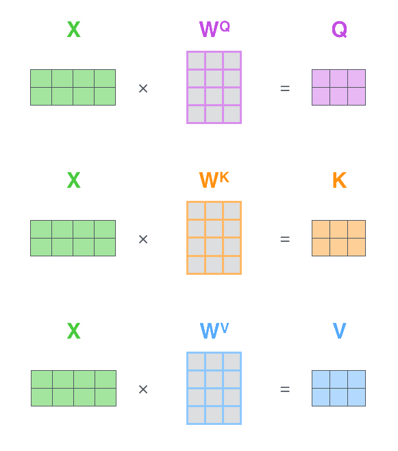Query, key, and value calculation in matrix form. From The Illustrated Transformer.Attention works by creating query $Q$, key $K$, and value $V$ matrices from inputs $X$ via linear layers with learnable weights $W^Q$, $W^K$, and $W^V$

$$Q=XW^Q \qquad K=XW^K \qquad V=XW^V$$

where $W^Q \in \R^{d_{model} \times d_Q}$. Or less formally, $Q = XW^Q$ is a set of linear equations $Q = XA^Q + B^Q$ where $A^Q$ and $B^Q$ are learnable parameters for calculating $Q$ from $X$.

Attention is then calculated by:

$$\tag{1}\mathrm{Attention}(Q, K, V) = \mathrm{softmax}\left(\frac{QK^T}{\sqrt{d_k}}\right)V$$

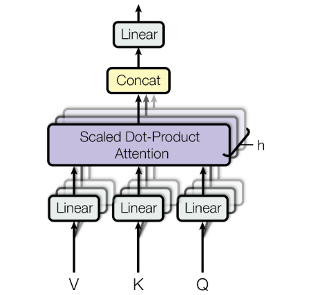
where $\sqrt{d_k}$ is a scaling factor, usually based on the individual head dimensionFor most Transformer implementations, $Q$, $K$, and $V$ all have the same shape. or number of heads.

This process is illustrated by Jay Alammar in Figure 1 on the rightFigure 1 is above if reading on mobile. and Figure 2 below.

Self-attention calculation in matrix form with attention denoted as $Z$. From The Illustrated Transformer.

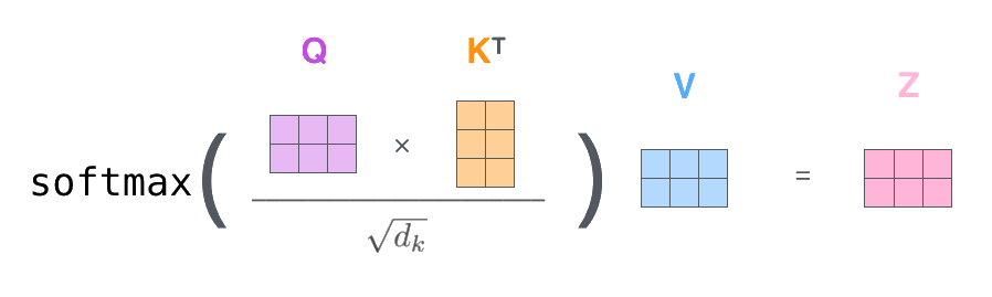
The resulting $\mathrm{Attention}(Q, K, V)$ is usually passed through a linear layer $W^O$ projection

$$\mathrm{Output} = \mathrm{Attention}(Q, K, V)W^O$$

as the final step of the Attention layer.

For all the math, Attention is simply a learned weighted average. Attention learns to generate weights between tokens via queries $XW^Q$ and keys $XW^K$. Those per-token weights are created by $\mathrm{softmax}(QK^T/\sqrt{d_k})$. The values $XW^V$ learn to create a token representation which can incorporate the weighted average of all the other tokens in the final dot product in the Attention layer $\mathrm{softmax}(...)V$. When someone says a token attends to a second token, this means it’s increasing the size of the second token’s weight in the weighted average relative to all the other tokens.

# Three Flavors of Attention

The three standard types of Attention layers introduced in Attention is All You Need, are Bidirectional Attention, Causal Attention, and Cross AttentionBidirectional Attention can also be referred as “fully-visible” and Causal Attention as “Autoregressive”.. Both Bidirectional and Causal Attention are forms of Self-Attention, as they only apply Attention to one input sequence, while Cross Attention applies Attention on multiple inputsI will explain each type of Attention in detail with code later in the post, so don’t worry if this overview is a bit confusing..

Bidirectional Attention is used in encoder blocks in encoder-only models (BERTJacob Devlin, Ming-Wei Chang, Kenton Lee, and Kristina Toutanova. 2019. BERT: Pre-training of Deep Bidirectional Transformers for Language Understanding. In Proceedings of the 2019 Conference of the North American Chapter of the Association for Computational Linguistics: Human Language Technologies, Volume 1 (Long and Short Papers), 4171–4186. DOI:10.18653/v1/N19-1423) or encoder-decoder models (BARTMike Lewis, Yinhan Liu, Naman Goyal, Marjan Ghazvininejad, Abdelrahman Mohamed, Omer Levy, Ves Stoyanov, and Luke Zettlemoyer. 2020. BART: Denoising Sequence-to-Sequence Pre-training for Natural Language Generation, Translation, and Comprehension. In Proceedings of the 58th Annual Meeting of the Association for Computational Linguistics, 7871–7880. DOI:10.18653/v1/2020.acl-main.703). It allows the Attention mechanism to incorporate both prior and successive tokens, regardless of order. Bidirectional Attention is used when we want to capture context from the entire input, such as classification.

Causal Attention is used in decoder blocks in decoder-only models (GPTAlec Radford, Karthik Narasimhan, Tim Salimans, and Ilya Sutskever. 2018. Improving language understanding by generative pre-training. (2018). Retrieved from https://openai.com/research/language-unsupervised) or encoder-decoder models (BART). Unlike Bidirectional Attention, Causal Attention can only incorporate information from prior tokens into the current token. It cannot see future tokens. Causal Attention is used when we need to preserve the temporal structure or a sequence, such as generating a next token based on prior tokens.

Cross Attention is used in cross blocks in encoder-decoder models (BART). Unlike Bidirectional and Causal Self-Attention, Cross Attention allows the Attention mechanism to incorporate a different sequence of tokens to the current sequence of tokens. Cross Attention is used when we need to align two sequences, such as translating from one language or domain to another, or when we want to incorporate multiple input types into one model, such as text and images in diffusion models.

# Single Head Self-Attention

A diagram of Single Head Self-Attention, or Scaled Dot Product Attention, without the last linear projection. From Attention is All You Need.We’ll start our implementation of a Attention layer with the simplest Attention mechanism: Single Head Bidirectional Self-Attention.

Recall that we are implementing the following formal definition of Attention:

$$Q=XW^Q \qquad K=XW^K \qquad V=XW^V \\[0.5em] \mathrm{Attention}(Q, K, V) = \mathrm{softmax}\left(\frac{QK^T}{\sqrt{d_k}}\right)V \\[0.5em] \mathrm{Output} = \mathrm{Attention}(Q, K, V)W^O$$

With Single Head Attention formally defined, let’s implement it in code.

# Single Head Initialization

In a Transformer, each token is passed through the model as a vector. The hidden_size defines how wide the token vector is when it reaches the Attention mechanism.

Our Attention layers will allow disabling bias terms for linear layers since recent papers and models, such as CrammingJonas Geiping and Tom Goldstein. 2022. Cramming: Training a Language Model on a Single GPU in One Day. arXiv:2212.14034., PythiaStella Biderman, Hailey Schoelkopf, Quentin Anthony, Herbie Bradley, Kyle O’Brien, Eric Hallahan, Mohammad Aflah Khan, Shivanshu Purohit, USVSN Sai Prashanth, Edward Raff, Aviya Skowron, Lintang Sutawika, and Oskar van der Wal. 2023. Pythia: A Suite for Analyzing Large Language Models Across Training and Scaling. arXiv:2304.01373., and PaLMAakanksha Chowdhery, Sharan Narang, Jacob Devlin, Maarten Bosma, Gaurav Mishra, Adam Roberts, Paul Barham, Hyung Won Chung, Charles Sutton, Sebastian Gehrmann, Parker Schuh, Kensen Shi, Sasha Tsvyashchenko, Joshua Maynez, Abhishek Rao, Parker Barnes, Yi Tay, Noam Shazeer, Vinodkumar Prabhakaran, Emily Reif, Nan Du, Ben Hutchinson, Reiner Pope, James Bradbury, Jacob Austin, Michael Isard, Guy Gur-Ari, Pengcheng Yin, Toju Duke, Anselm Levskaya, Sanjay Ghemawat, Sunipa Dev, Henryk Michalewski, Xavier Garcia, Vedant Misra, Kevin Robinson, Liam Fedus, Denny Zhou, Daphne Ippolito, David Luan, Hyeontaek Lim, Barret Zoph, Alexander Spiridonov, Ryan Sepassi, David Dohan, Shivani Agrawal, Mark Omernick, Andrew M. Dai, Thanumalayan Sankaranarayana Pillai, Marie Pellat, Aitor Lewkowycz, Erica Moreira, Rewon Child, Oleksandr Polozov, Katherine Lee, Zongwei Zhou, Xuezhi Wang, Brennan Saeta, Mark Diaz, Orhan Firat, Michele Catasta, Jason Wei, Kathy Meier-Hellstern, Douglas Eck, Jeff Dean, Slav Petrov, and Noah Fiedel. 2022. PaLM: Scaling Language Modeling with Pathways. arXiv:2204.02311., have shown that disabling the bias term results in little-to-no downstream performance dropIn a well-trained NLP Transformer, such as Pythia, the bias term ends up being near or at zero, which is why we can disable them without causing performance issues. while decreasing computational and memory requirements. However, to match the original Transformer implementation, we will set it on by default.

class SingleHeadAttention(nn.Module):
    def __init__(self,
        hidden_size: int,
        bias: bool = True,
    ):

In this implementation, we will start merge $W^Q$, $W^K$, and $W^V$ into single linear layer, Wqkv, and unbind the outputs into $Q$, $K$, and $V$. This is accomplished by increasing the output shape by a factor of threeAlternatively, we might use two layers, one for $Q$ and one for both $K$ and $V$ for implementing $KV$ caching.. This is mathematically equivalent to three individual linear layers, each with the same input and output shape.

In Multi-Head Attention, each individual head size is smaller than the input sizeThis reduction to forces $W^Q$, $W^K$, and $W^V$ to learn a condensed representation of the input tokens., so for Single Head we will arbitrarily set the head size to be four times smaller than the input dimension.

# linear layer to project queries, keys, values
Wqkv = nn.Linear(hidden_size, (hidden_size//4)*3, bias=bias)

Like the Wqkv layer, the Attention layer’s linear projection layer also has an optional bias term. In the Single Head setting, it also projects the attended tokens back to the original shape.

# linear layer to project final output
proj = nn.Linear(hidden_size//4, hidden_size, bias=bias)

And that’s it for the Attention initialization. The Attention mechanism in a Transformer only has twoOr four if $W^Q$, $W^K$, and $W^V$ are all separate linear layers. layers of learnable parameters. Everything else in Attention is an operation on the output of the Wqkv linear layer.

def __init__(self,
    hidden_size: int,
    bias: bool = True,
):
    super().__init__()
    self.Wqkv = nn.Linear(hidden_size, (hidden_size//4)*3, bias=bias)
    self.Wo = nn.Linear(hidden_size//4, hidden_size, bias=bias)

With our linear projection layers created, we can now move to the forward method of the Attention layer.

# Single Head Forward

After some input shape housekeeping, the first computational step is to generate our keys, queries, and values. First, we pass the input x through the Wqkv linear layer. Then we reshape the Wqkv output to batch size, sequence length, one dimension for $Q$, $K$, & $V$, and the head size Which in this example is the hidden size divided by four.. Finally, we split the single tensor into the query, key, and value tensors using unbind, where each are of shape B, S, C//4.

# batch size (B), sequence length (S), input dimension (C)
B, S, C = x.shape

# split into queries, keys, & values of shape
# batch size (B), sequence length (S), head size (HS)
q, k, v = self.Wqkv(x).reshape(B, S, 3, C//4).unbind(dim=2)

With the queries, keys, and values generatedInstead of reshape(...).unbind(2) we could also use einops: rearrange(x, "b s (qkv c) -> qkv b s c", qkv=3). Although it may be slower then using PyTorch ops., we can move to the mathematical operations of the Attention mechanism.

Remember that Attention is defined by this equation:

$$\mathrm{Attention}(Q, K, V) = \mathrm{softmax}\left(\frac{QK^T}{\sqrt{d_k}}\right)V$$

So first, we need to transpose $K$ and take the dot product of $Q$ and $K^T$.

# calculate dot product of queries and keys of shape
# (B, S, S) = (B, S, HS) @ (B, HS, S)
attn = q @ k.transpose(-2, -1)

Next, we need to scale the outputs of the $QK^T$ by $\sqrt{d_k}$

# scale by square root of head dimension
attn = attn / math.sqrt(k.size(-1))

Now that we have scaled $QK^T$, it’s time to calculate the token Attention weight using softmax.

# apply softmax to get attention weights
attn = attn.softmax(dim=-1)

Single Head Self-Attention weights on a sequence of tokens. Darker shading means a higher Self-Attention weight. From The Illustrated Transformer. This Softmax output of $QK^T/\sqrt{d_k}$ is how the Attention mechanism weights the strength of the relationship between each pair of tokens. Where higher Softmax values means Attention is placing more importance on these pairs of tokens and lower values are deemed less important.

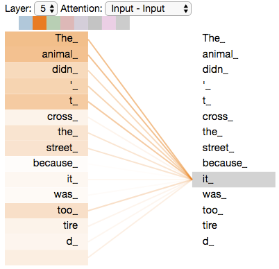
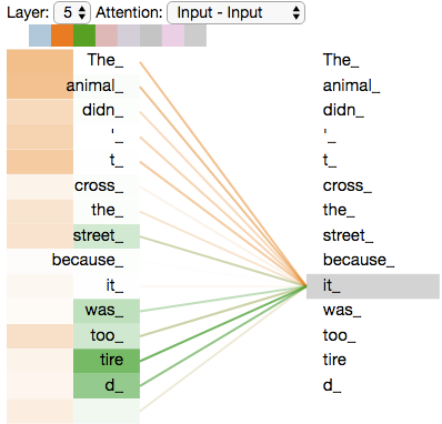
This is illustrated in figure 3, where the Attention mechanism has learned to associate the word “it” to “animal” in the sentence, “the animal didn’t cross the street because it was too tired.”

Next we matrix multiply the Attention weights with our value matrix $V$ which applies the Attention weights to our propagating token embeddingsRemember that $V$ is of shape B, S, HS, where S, HS are the projected token embeddings for our sequence of length S..

# dot product attention weights to values
# (B, S, HS) = (B, S, S) @ (B, S, HS)
x = attn @ v

Finally, we project the Attention results through the final linear layer to get the Attention layer output, which is back to the input shape.

# apply final linear layer to get output (B, S, C)
return self.Wo(x)

And there you have it. A simple rendition of Single Head Bidirectional Attention in code.

class SingleHeadAttention(nn.Module):
    def __init__(self,
        hidden_size: int,
        bias: bool = True,
    ):
        super().__init__()
        self.Wqkv = nn.Linear(hidden_size, (hidden_size//4)*3, bias=bias)
        self.Wo = nn.Linear(hidden_size//4, hidden_size, bias=bias)

    def forward(self, x:Tensor):
        B, S, C = x.shape

        q, k, v = self.Wqkv(x).reshape(B, S, 3, C//4).unbind(dim=2)

        attn = q @ k.transpose(-2, -1)
        attn = attn / math.sqrt(k.size(-1))

        attn = attn.softmax(dim=-1)

        x = attn @ v

        return self.Wo(x)

# Multi-Head Self-Attention

Two-head Self-Attention weights on a sequence of tokens. Darker shading means a higher Self-Attention weight. From The Illustrated Transformer.Now that we have our Single Head Self-Attention code understood and working, we can update it to Bidirectional Multi-Head Self-Attention. But first, there is an obvious question which needs to be answered: Why do we want Multi-Head Attention in the first place?

The answer is two parted. First, by projecting the input to multiple randomly initialized heads the Transformer will have multiple representation subspaces for the same input, giving each Transformer layer the ability to simultaneously learn different nuances for the same input tokens.

Second, multiple heads allow the Attention mechanism to jointly attended to multiple tokens at the same timeAlthough there is a paper which suggests that enough layers of Single Head Attention can perform the same function.. Even if a single weighted average is well behavedA worst case scenario for a Single Headed Attention is the Softmax output only attends to itself or one other token, with all the other tokens contributing a miniscule amount., it still limits the ability to focus on multiple tokens. This ability to attend to multiple tokens at once is especially important as the context windowThe context window is the maximum number of tokens in the input sequence that the model was trained or fine-tuned on. of recent LLMs expands to 4,000, 8,000, 32,000, 60,000, and even 100,000 tokens.

A diagram of Multi-Head Self-Attention where each Scaled Dot Product Attention is per head Single Head Attention. From Attention is All You Need.Formally, Multi-Head Attention creates one query $Q_h$, key $K_h$, and value $V_h$ per head $h$, calculates the scaled dot-product Attention per head $\mathrm{Attention}(Q_h, K_h, V_h)$, concatenates all the Attention outputs back into one tensor $\mathrm{MultiHead}(Q, K, V)$, before passing the Multi-Head Attention output through the final linear layer $W^O$:

$$Q_h=XW_h^Q \qquad K_h=XW_h^K \qquad V_h=XW_h^V \\[0.5em] \mathrm{Attention}(Q_h, K_h, V_h) = \mathrm{softmax}\left(\frac{Q_hK_h^T}{\sqrt{d_h}}\right)V_h \\[0.5em] \mathrm{MultiHead}(Q, K, V) = \mathrm{concat}(\mathrm{Attention}(Q_h, K_h, V_h), \text{ for all } h) \\[0.5em] \mathrm{Output} = \mathrm{MultiHead}(Q, K, V)W^O$$

With Multi-Head Attention formally defined, let’s implement it in code.

# Multi-Head Initialization

Our Multi-Head Attention __init__ will look quite similar to the Single Head implementation, except with a new argument num_heads to set the number of heads.

class MultiHeadAttention(nn.Module):
    def __init__(self,
        hidden_size: int,
        num_heads: int,
        bias: bool = True,
    ):

Instead of projecting the input to a fixed size like in Single Head Attention, we will project the input to hidden_size / num_heads, so we want to assert that the shapes match.

# input dimension must be divisible by num_heads
assert hidden_size % num_heads == 0
# number of attention heads
self.nh = num_heads

We now have all the learnable parameters for our Multi-Head Attention mechanismSince each head is a subset of the hidden_size, we can remove the projection reduction added to Single Head Attention..

def __init__(self,
    hidden_size: int,
    num_heads: int,
    bias: bool = True,
):
    # input dimension must be divisible by num_heads
    assert hidden_size % num_heads == 0
    # number of attention heads
    self.nh = num_heads
    super().__init__()
    # linear layer to project queries, keys, values
    self.Wqkv = nn.Linear(hidden_size, hidden_size*3, bias=bias)
    # linear layer to project final output
    self.Wo = nn.Linear(hidden_size, hidden_size, bias=bias)

# Multi-Head Forward

Our Multi-Head forward method is largely the same, with a few changes to account for the multiple heads.

Our input sequence is projected through the linear Wqkv layer as before. Then we need to reshape and transpose the output to batch size, number of heads, $Q_h$, $K_h$, & $V_h$, sequence length, and the head size, which in most Transformers is the embedding shape divided by the number of heads. Then we unbind our reshaped and transposed output to the separate queries, keys, & values, each of shape B, NH, S, HSLike the Single Head Attention, we could also use einops: rearrange(x, "b s (qkv nh hs) -> qkv b nh s hs", qkv=3, nh=self.nh). Although it may be slower than using PyTorch ops..

# batch size (B), sequence length (S), input dimension (C)
B, S, C = x.shape

# split into queries, keys, & values of shape
# batch size (B), num_heads (NH), sequence length (S), head size (HS)
x = self.Wqkv(x).reshape(B, S, 3, self.nh, C//self.nh)
q, k, v = x.transpose(3, 1).unbind(dim=2)

The Attention mechanism is exactly the same as the Single Head code, but the difference in tensor shape means we are calculating the Softmax individually per each headThe input shape at the Softmax layer is B, NH, S, S and we are applying it on the last dimension..

# calculate dot product of queries and keys
# (B, NH, S, S) = (B, NH, S, HS) @ (B, NH, HS, S)
attn = q @ k.transpose(-2, -1)

# scale by square root of head dimension
attn = attn / math.sqrt(k.size(-1))

# apply softmax to get attention weights
attn = attn.softmax(dim=-1)

Our remaining steps are to matrix multiply the Attention outputs with $V_h$, then concatenate the per-head Attention into one output of our input shape.

We perform this by transposing the heads and sequences then reshaping to B, S, CWe could also use einops: rearrange(x, "b nh s hs -> b s (nh hs)").. This is mechanically the same as a concatenation, without the requirement of creating a new tensorAlong with the expensive increase in memory and read+write.

# dot product attention weights with values
# (B, NH, S, HS) = (B, NH, S, S) @ (B, NH, HS, S)
x = attn @ v

# transpose heads & sequence then reshape back to (B, S, C)
x = x.transpose(1, 2).reshape(B, S, C)

# apply final linear layer to get output
return self.Wo(x)

With all the pieces defined, we now have a working, albeit incomplete, implementation of Bidirectional Self-Attention.

class MultiHeadAttention(nn.Module):
    def __init__(self,
        hidden_size: int,
        num_heads: int,
        bias: bool = True,
    ):
        super().__init__()
        assert hidden_size % num_heads == 0
        self.nh = num_heads
        self.Wqkv = nn.Linear(hidden_size, hidden_size * 3, bias=bias)
        self.Wo = nn.Linear(hidden_size, hidden_size, bias=bias)

    def forward(self, x: Tensor):
        B, S, C = x.shape

        x = self.Wqkv(x).reshape(B, S, 3, self.nh, C//self.nh)
        q, k, v = x.transpose(3, 1).unbind(dim=2)

        attn = q @ k.transpose(-2, -1)
        attn = attn / math.sqrt(k.size(-1))

        attn = attn.softmax(dim=-1)

        x = attn @ v

        return self.Wo(x.transpose(1, 2).reshape(B, S, C))

Technically, we could use this in an encoder model like BERT, but there are a few more items we need to define before all the original Attention is All You Need Bidirectional Self-Attention is fully recreated.

# Adding Dropout

The original Attention Is All You Need Attention implementation has dropout for both the Attention weights and the final projection layer. They are simple to add, with a default dropout probability of 10 percent.

def __init__(self,
    hidden_size: int,
    num_heads: int,
    attn_drop: float = 0.1,
    out_drop: float = 0.1,
    bias: bool = True,
):
    super().__init__()
    assert hidden_size  % num_heads == 0
    self.nh = num_heads
    self.Wqkv = nn.Linear(hidden_size, hidden_size * 3, bias=bias)
    self.Wo = nn.Linear(hidden_size, hidden_size, bias=bias)
    # attention dropout layer to prevent overfitting
    self.attn_drop = nn.Dropout(attn_drop)
    # final output dropout layer to prevent overfitting
    self.out_drop = nn.Dropout(out_drop)

The Attention dropout is placed directly after the Attention Softmax is calculated. Note that this will completely remove whole tokens from the Attention weightsHugging Face implementations note that this seems odd, but it’s what Attention Is All You Need does., as the shape is B, NH, S, S.

# apply softmax to get attention weights (B, NH, S, S)
attn = attn.softmax(dim=-1)

# apply dropout to attention weight
attn = self.attn_drop(attn)

The final projection layer dropout is applied after the projection layer is calculated, and it removes a fraction of the token embedding activations, not tokens themselves.

# apply final linear layer to get output (B, S, C)
return self.out_drop(self.Wo(x))

# Bidirectional Attention

The last thing our Bidirectional Multi-Head Self-Attention layer needs to be complete is the input Attention mask.

As Bidirectional Attention is supposed to attend to all tokens in the input sequence, the Attention mask primarily exists to support batching different length sequencesAlthough with Nested Tensors on the horizon, the necessity of masking might diminish.. Typically, an encoder or encoder-decoder Transformer will have a pad token, but we don’t want this pad token to interact with any of the sequence tokens. That is where the Attention mask comes in.

# boolean mask of shape (batch_size, sequence_length)
# where True is masked and False is unmasked
def forward(self, x: Tensor, mask: BoolTensor):

Our Attention mask is applied right before the Softmax calculates the Attention weights. For simplicity and conciseness, we are requiring a mask to be passed to the Attention layer.

# scale by square root of output dimension
attn = attn / math.sqrt(k.size(-1))

# reshape and mask attention scores
attn = attn.masked_fill(mask.view(B, 1, 1, S), float('-inf'))

# apply softmax to get attention weights
attn = attn.softmax(dim=-1)

By setting the padding tokens to a value of negative infinityPyTorch will take care of converting this to the correct value if we are training in mixed precision with autocast. this means softmax will weight these tokens as zero when calculating the Attention results.

The entire BidirectionalAttention layer can be seen below, with a fully commented version in commented-transformers.

class BidirectionalAttention(nn.Module):
    def __init__(self,
        hidden_size: int,
        num_heads: int,
        attn_drop: float = 0.1,
        out_drop: float = 0.1,
        bias: bool = True,
    ):
        super().__init__()
        assert hidden_size % num_heads == 0
        self.nh = num_heads
        self.Wqkv = nn.Linear(hidden_size, hidden_size * 3, bias=bias)
        self.Wo = nn.Linear(hidden_size, hidden_size, bias=bias)
        self.attn_drop = nn.Dropout(attn_drop)
        self.out_drop = nn.Dropout(out_drop)

    def forward(self, x: Tensor, mask: BoolTensor):
        B, S, C = x.shape

        x = self.Wqkv(x).reshape(B, S, 3, self.nh, C//self.nh)
        q, k, v = x.transpose(3, 1).unbind(dim=2)

        attn = q @ k.transpose(-2, -1)

        attn = attn / math.sqrt(k.size(-1))
        attn = attn.masked_fill(mask.view(B, 1, 1, S), float('-inf'))

        attn = attn.softmax(dim=-1)
        attn = self.attn_drop(attn)

        x = attn @ v

        x = x.transpose(1, 2).reshape(B, S, C)
        return self.out_drop(self.Wo(x))

# Causal Self-Attention

An illustration of causal masking on a single input sequence. Gray shading indicates a masked token. From The Illustrated GPT2.For Causal Attention, we need to ensure that current tokens can only attend to past tokens, and not future tokens in the sequence. We can accomplish this through masking.

We will use an upper triangular matrix for the Causal Attention mask to ensure the current token can only attend to past tokens no matter where the current token is in the sequence. Figure 7 illustrates how the upper triangular matrix is applied on a per-token level, where the diagonal, $(1,1)$, $(2,2)$, etc, is the current token in the sequence. Green shaded tokens, both the current token and tokens to the left of the current token, are unmasked and can be attended too, while grey shaded tokens to the right of the current token are masked and cannot used in the Attention mechanism.

We’ll create a permanent causal_mask of shape [context_size, context_size] in our CausalAttention initialization method, where context_size is the maximum context length of our Transformer. To match our padding Attention maskWhere True is masked and False is unmasked. we will create a matrix of boolean ones. Then we use triu to convert our boolean matrix of True values into an upper triangular matrix, with the upper triangle masked (True) and lower triangle unmasked (False). Because we want the diagonal of the matrix to be unmasked, we shift the triu diagonal one to the upper-right using diagonal=1.

Then we reshape the input to be broadcastable across the dimensions of $QK^{T}$, which is B, NH, S, S, and assign it to a PyTorch bufferThis insures the values are not considered parameters, and thus will not be modified by an optimizer..

# causal mask to ensure that attention is not applied to future tokens
# where context_size is the maximum sequence length of the transformer
self.register_buffer('causal_mask',
    torch.triu(torch.ones([context_size, context_size],
               dtype=torch.bool), diagonal=1)
        .view(1, 1, context_size, context_size))

Then in our CausalAttention forward method, we use masked_fill again to apply the causal mask to our intermediate Attention results before applying softmax to calculate the Attention weights.

# scale by square root of output dimension
attn = attn / math.sqrt(k.size(-1))

# apply causal mask
attn = attn.masked_fill(self.causal_mask[:, :, :S, :S], float('-inf'))

# apply softmax to get attention weights
attn = attn.softmax(dim=-1)

We can also combine the causal Attention masking with our input Attention mask. Since both masks are booleanIn boolean addition, True + False = True, and adding True or False to themselves results in no change., we can add them together thanks to PyTorch broadcasting.

# apply input and causal mask
combined_mask = self.causal_mask[:, :, :S, :S] + mask.view(B, 1, 1, S)
attn = attn.masked_fill(combined_mask, float('-inf'))

With those two changes, we have modified Bidirectional Attention into Causal Attention. The entire CausalAttention layer can be seen below, with a fully commented version in commented-transformers.

class CausalAttention(nn.Module):
    def __init__(self,
        hidden_size: int,
        num_heads: int,
        context_size: int,
        attn_drop: float = 0.1,
        out_drop: float = 0.1,
        bias: bool = True,
    ):
        super().__init__()
        assert hidden_size % num_heads == 0
        self.nh = num_heads
        self.Wqkv = nn.Linear(hidden_size, hidden_size * 3, bias=bias)
        self.Wo = nn.Linear(hidden_size, hidden_size, bias=bias)
        self.attn_drop = nn.Dropout(attn_drop)
        self.out_drop = nn.Dropout(out_drop)
        self.register_buffer('causal_mask',
            torch.triu(torch.ones([context_size, context_size],
                       dtype=torch.bool), diagonal=1)
                .view(1, 1, context_size, context_size))

    def forward(self, x: Tensor, mask: BoolTensor):
        B, S, C = x.shape

        x = self.Wqkv(x).reshape(B, S, 3, self.nh, C//self.nh)
        q, k, v = x.transpose(3, 1).unbind(dim=2)

        attn = q @ k.transpose(-2, -1)
        attn = attn / math.sqrt(k.size(-1))

        combined_mask = self.causal_mask[:, :, :S, :S] + mask.view(B, 1, 1, S)
        attn = attn.masked_fill(combined_mask, float('-inf'))

        attn = attn.softmax(dim=-1)
        attn = self.attn_drop(attn)

        x = attn @ v

        x = x.transpose(1, 2).reshape(B, S, C)
        return self.out_drop(self.Wo(x))

# Cross Attention

All of the versions of Attention we’ve covered so far have been implementations of Self-Attention, which is applying the Attention mechanism on the same input sequence. Cross Attention differs from Self-Attention in that the Attention mechanism applies across more than one input sequences.

This means our formal definition of Attention needs some modifications. For this post, I will follow the original Cross Attention implementation, where the query is created from the first sequence $X$ and both the keys and values are from the second sequence $Y$. However, these are not set in stone, with other Transformer models adopting different allocations of the first and second sequence across the queries, keys, and values.

The formal definition for Cross Attention is the sameFor conciseness, I removed the separate concatenation step and bundled it into the $\mathrm{CrossAttention}$ operation., but with $Q_X$, $K_Y$, and $V_Y$ representing the Multi-Head queries, keys, and values for inputs $X$ and $Y$, respectively.

$$Q_X=XW_h^Q \qquad K_Y=YW_h^K \qquad V_Y=YW_h^V \\[0.5em] \mathrm{CrossAttention}(Q_X, K_Y, V_Y) = \mathrm{softmax}\left(\frac{Q_XK_Y^T}{\sqrt{d_h}}\right)V_Y \\[0.5em] \mathrm{Output} = \mathrm{CrossAttention}(Q_X, K_Y, V_Y)W^O$$

Our Cross Attention __init__ method differs from prior initializations due to requiring separate linear layers for queries and the keys and values.

# linear layer to project queries from decoder input
self.Wq = nn.Linear(hidden_size, hidden_size, bias=bias)
# linear layer to project keys and values from encoder output
self.Wkv = nn.Linear(hidden_size, hidden_size * 2, bias=bias)

Our new forward method has two sequence inputs along with the mask. The decoder input $X$, and the encoder input $Y$. We’ll assume for sake of simplicity and code reuse that both inputs are the same shape.

def forward(self, x: Tensor, y: Tensor, mask: BoolTensor):
    # batch size, sequence length, input dimension
    B, S, C = x.shape

    # split into queries of shape (B, NH, S, HS) from decoder input
    q = self.Wq(x).reshape(B, S, self.nh, C//self.nh).transpose(1, 2)

    # split into keys and values of shape (B, NH, S, HS) from encoder output
    y = self.Wkv(y).reshape(B, S, 2, self.nh, C//self.nh)
    k, v = y.transpose(3, 1).unbind(dim=2)

Since we are assuming this Cross Attention is in the decoder side of an encoder-decoder transformer, everything after creating the queries, keys, and values is the same as our Causal Attention implementation.

If we were creating Cross Attention for an encoder style Attention layer, we would remove the causal mask and optionally keep the input mask if appropriate for our task.

The entire CausalCrossAttention layer can be seen below, with a fully commented version in the commented-transformers.

class CausalCrossAttention(nn.Module):
    def __init__(self,
        hidden_size: int,
        num_heads: int,
        context_size: int,
        attn_drop: float = 0.1,
        out_drop: float = 0.1,
        bias: bool = True,
    ):
        super().__init__()
        assert hidden_size % num_heads == 0
        self.nh = num_heads
        self.Wq = nn.Linear(hidden_size, hidden_size, bias=bias)
        self.Wkv = nn.Linear(hidden_size, hidden_size * 2, bias=bias)
        self.Wo = nn.Linear(hidden_size, hidden_size, bias=bias)
        self.attn_drop = nn.Dropout(attn_drop)
        self.out_drop = nn.Dropout(out_drop)
        self.register_buffer('causal_mask',
            torch.triu(torch.ones([context_size, context_size],
                       dtype=torch.bool), diagonal=1)
                .view(1, 1, context_size, context_size))

    def forward(self, x: Tensor, y: Tensor, mask: BoolTensor):
        B, S, C = x.shape

        q = self.Wq(x).reshape(B, S, self.nh, C//self.nh).transpose(1, 2)
        y = self.Wkv(y).reshape(B, S, 2, self.nh, C//self.nh)
        k, v = y.transpose(3, 1).unbind(dim=2)

        attn = q @ k.transpose(-2, -1)
        attn = attn / math.sqrt(k.size(-1))

        combined_mask = self.causal_mask + mask.view(B, 1, 1, S)
        attn = attn.masked_fill(combined_mask, float('-inf'))

        attn = attn.softmax(dim=-1)
        attn = self.attn_drop(attn)

        x = attn @ v

        x = x.transpose(1, 2).reshape(B, S, C)
        return self.out_drop(self.Wo(x))

# Conclusion

In this post, I have shown you how to implement all three main flavors of Attention in PyTorch: Bidirectional, Causal, and Cross Attention. You should now be able to write your own version of Attention and understand any model-specific Attention implementations.

There still are a few more items we need to create before we have a fully working Transformer: the feed-forward network, positional encoding, and text embedding layers, to name a few. In the next post in this series, I will show you how to create all of these in PyTorch and build the rest of the Transformer.