Transformers are everywhere. They are the backbone of modern language models like ChatGPT. Transformers power the state-of-the-art voice to text models such as Whisper. In most domains, Transformers are giving other model architectures a run for their money.
But what exactly is a Transformer and how does it work under the hood?
Code for this post can be found here: commented-transformers.This is the second post in a multi-part series on creating a Transformer from scratch in PyTorch. By the end of the series, you will be familiar with the architecture of a standard Transformer and common variants you will find across recent models such as GPT, PaLM, LLaMA, MPT, and Falcon. You will also be able to understand how Transformers are being used in domains other then language.
In the previous post in this series, I showed you how to create the three main flavors of Attention: Bidirectional, Causal, and Cross Attention. In this post, I will show you how to build the rest of the Transformer. By the end you will be familiar with all the pieces of a Transformer model and, combined with your knowledge of Attention, will be able to write an entire Transformer from scratch.
# Transformer Layers
The heart of a Transformer is a stack of multiple Transformer layers, or blocks. In a standard Transformer, each block has two components: the Attention mechanism and the Feed Forward Network.
The first part of the Transformer layer is Attention. Specifically, Multi-Head AttentionOr Multi-Head Attention varients..
We created the three main versions of Attention, Bidirectional, Causal, and Cross Attention, in the previous post in this seriesIf this formal definition looks unfamiliar, I’d recommend giving it a read before continuing..
The second part of the Transformer layer is the Feed Forward Network, or Multilayer Perceptron. We’ll define the Feed Forward Network next, then resume creating the standard Transformer Block. Then we will define vocabulary and positional embeddings and finish by building both a GPT-2Alec Radford, Karthik Narasimhan, Tim Salimans, and Ilya Sutskever. 2018. Improving language understanding by generative pre-training. (2018). Retrieved from https://openai.com/research/language-unsupervised decoder-only model and BERTJacob Devlin, Ming-Wei Chang, Kenton Lee, and Kristina Toutanova. 2019. BERT: Pre-training of Deep Bidirectional Transformers for Language Understanding. In Proceedings of the 2019 Conference of the North American Chapter of the Association for Computational Linguistics: Human Language Technologies, Volume 1 (Long and Short Papers), 4171–4186. DOI:10.18653/v1/N19-1423 encoder-only model from scratch.
# Feed Forward Network
Unlike the Attention layer, the Feed Forward Network (Feed Forward or FFN) operates on each token independently of all other tokens in the sequence. It cannot reference other tokens or positional information outside of the information embedded in the current token vector.
Formally, the Feed Forward layer is defined as
where is a linear layer which projects token vectors into a higher dimensional space , is the activation functionMost modern Transformers use GeLU, or a Gated Linear Unit (GLU) with GeLU. Google likes to use SiLU and GLU-SiLU. ReLU and Softmax also make appearances from time to time. GLU will be covered in a future post in this series., and projects the expanded token vectors back down to the input space .
The Feed Forward Network can be thought providing an implicit key-value memoryMor Geva, Roei Schuster, Jonathan Berant, and Omer Levy. 2021. Transformer Feed-Forward Layers Are Key-Value Memories. In Empirical Methods in Natural Language Processing (EMNLP). to the Transformer layer, with the upscaling projection generating per-token keys into the FFN’s working memory. Neurons in the Feed Forward layers are thought to be polysemantic, responding to multiple concepts at once. The superposition hypothesis suggests the neuron’s polysemanticity simulates a much larger layerChris Olah, Nick Cammarata, Ludwig Schubert, Gabriel Goh, Michael Petrov, and Shan Carter. 2020. Zoom In: An Introduction to Circuits. Distill (2020). DOI:10.23915/distill.00024.001, which allows the model to understand more features then parameters.
The Softmax Linear UnitsNelson Elhage, Tristan Hume, Catherine Olsson, Neel Nanda, Tom Henighan, Scott Johnston, Sheer ElShowk, Nicholas Joseph, Nova DasSarma, Ben Mann, Danny Hernandez, Amanda Askell, Kamal Ndousse, And Jones, Dawn Drain, Anna Chen, Yuntao Bai, Deep Ganguli, Liane Lovitt, Zac Hatfield-Dodds, Jackson Kernion, Tom Conerly, Shauna Kravec, Stanislav Fort, Saurav Kadavath, Josh Jacobson, Eli Tran-Johnson, Jared Kaplan, Jack Clark, Tom Brown, Sam McCandlish, Dario Amodei, and Christopher Olah. 2022. Softmax Linear Units. Transformer Circuits Thread (2022). Retrieved from https://transformer-circuits.pub/2022/solu/index.html interpretability study by Elhage et al found that early, middle, and late Feed Forward layers likelyElhage et al describe their work as preliminary and requiring more detailed follow-up study. The study also changes the activation function used in most Transformers, which could modify the results. focus on different aspects of language modeling. Early layers are often involved in “detokenizing” inputs into discrete concepts, with neurons which recognize multi-token words, names of famous people, compound words, programming commands, and related nounsRemember that after the first Attention layer, each individual token can be a combination of multiple tokens due to the Attention mechanism. This does not violate the FFN operating on each token individually.. Middle layers tend to respond to abstract ideas. Elhage et al highlight examples such as any clause which describes music, numbers of people, and discourse markers. The final layers of the model tend to focus on converting the discrete concepts back into individual tokens.
# Feed Forward Implementation
Since the Feed Forward Network is two Linear layers with an activation function in-between, it is easy to implement. The first Linear layer projects the token vector from the input size to the expanded size, and the second Linear layer reverses the projection back to the input size. In this implementation I place an optional dropout layer after the last linear layer. Some models place it before the last linear layer.
Like the Attention layer, our Linear layers in the Feed Forward layer will optionally allow the biases to be disabled for increased throughput and reduced memory usage.
class FeedForward(nn.Module):
    def __init__(self,
        hidden_size:int,
        expand_size:int,
        act:nn.Module=nn.GELU,
        drop:float=0.1,
        bias:bool=True,
    ):
        super().__init__()
        # project input to expanded dimension
        self.fc1 = nn.Linear(hidden_size, expand_size, bias=bias)
        # activation function to introduce non-linearity
        self.act = act()
        # project back to the input dimension
        self.fc2 = nn.Linear(expand_size, hidden_size, bias=bias)
        # optional dropout layer to prevent overfitting
        self.drop = nn.Dropout(drop)

    def forward(self, x:Tensor):
        x = self.fc1(x) # apply first linear layer
        x = self.act(x) # apply activation function
        x = self.fc2(x) # apply second linear layer
        x = self.drop(x) # optionally apply dropout layer
        return x
# Transformer Block
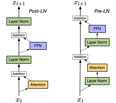
Post-Norm was introducedAlthough this doesn’t match the updated official implementation. in Attention is All You NeedAshish Vaswani, Noam Shazeer, Niki Parmar, Jakob Uszkoreit, Llion Jones, Aidan N. Gomez, Lukasz Kaiser, and Illia Polosukhin. 2017. Attention is All You Need. In Proceedings of the 31st International Conference on Neural Information Processing Systems (NIPS’17), 6000–6010., and was used in prominent early follow-up models such as BERT. Post-Norm applies the normalization layer to both the Attention/Feed Forward layer and residual connection.
Post-Norm can suffer from gradient vanishing as normalization is applied to the outputs of initial layers multiple timesDue to the residual connections being normalized.. Xiong et alYunchang Yang, Di He, Kai Zheng, Shuxin Zheng, Chen Xing, Huishuai Zhang, Yanyan Lan, Liwei Wang, Tieyan Liu, and Xiong. 2020. On Layer Normalization in the Transformer Architecture. In Proceedings of the 37th International Conference on Machine Learning (Proceedings of Machine Learning Research), 10524–10533. Retrieved from https://proceedings.mlr.press/v119/xiong20b.html show that this can cause the gradient norm to become exponentially small which hinders model training. Using small learning rates and learning rate warmup improves Post-Norm trainingToan Q. Nguyen and Julian Salazar. 2019. Transformers without Tears: Improving the Normalization of Self-Attention. In Proceedings of the 16th International Conference on Spoken Language Translation, Association for Computational Linguistics. Retrieved from https://aclanthology.org/2019.iwslt-1.17.
Wang et alQiang Wang, Bei Li, Tong Xiao, Jingbo Zhu, Changliang Li, Derek F. Wong, and Lidia S. Chao. 2019. Learning Deep Transformer Models for Machine Translation. In Proceedings of the 57th Annual Meeting of the Association for Computational Linguistics, ACL, 1810–1822. DOI:10.18653/v1/P19-1176 brought Pre-Norm from RNNs to Transformers. Pre-Norm applies the normalization layer to the input before it’s passed to the Attention and Feed Forward layers.
Pre-Norm has its own potential drawback of representational collapseLiyuan Liu, Xiaodong Liu, Jianfeng Gao, Weizhu Chen, and Jiawei Han. 2020. Understanding the difficulty of training transformers. arXiv:2004.08249., where the last model layersThose closest to the model output. will be highly similar to each other, contributing little to model capacity. However, Xiong et al show that Pre-Norm Transformers can train faster than Post-Norm due to stable gradient flow between layers. This allows higher learning rates and reduces the need for learning rate warmup.
Due to the benefits of training speed and stability, most modern Transformer-baed Large Language Models use Pre-Norm or a variation of Pre-NormFor example, GPT, T5, Cramming BERT, MPT, and Falcon all use Pre-Norm. And GPT-J, GPT-NeoX, and PaLM use Pre-Norm with their Parallel Transformer Block..
# Transformer Block Implementation
The initialization of the Transformer Block layer combines an Attention layer, which could be one of Bidirectional , Causal, or Cross Attention, with the Feed Forward layer and the two normalization layers.
This __init__ assumes the Transformer layer will Pre-Norm. If Post-Norm, we’d want to initialize the normalization layers after Attention and FeedForward so PyTorch would display them in the correct location.
class TransformerBlock(nn.Module):
    def __init__(self,
        hidden_size:int,
        num_heads:int,
        context_size:int,
        expand_size:int,
        attention:nn.Module=CausalAttention,
        act:nn.Module=nn.GELU,
        attn_drop:float=0.1,
        out_drop:float=0.1,
        ffn_drop:float=0.1,
        bias:bool=True,
    ):
        super().__init__()
        self.norm1 = nn.LayerNorm(hidden_size)
        self.attn = attention(
            hidden_size=hidden_size,
            num_heads=num_heads,
            context_size=context_size,
            attn_drop=attn_drop,
            out_drop=out_drop,
            bias=bias
        )
        self.norm2 = nn.LayerNorm(hidden_size)
        self.ffn = FeedForward(
            hidden_size=hidden_size,
            expand_size=expand_size,
            act=act,
            drop=ffn_drop,
            bias=bias,
        )
Both Pre-Norm and Post-Norm forward methods are simple to code. Remember that Post-Norm applies the normalization layer to both the Attention/Feed Forward layer and residual connection.
def forward(self, x: Tensor):
    # normalize residual connection and attention output
    x = self.norm1(x + self.attn(x))
    # normalize residual connection and feedforward output
    return self.norm2(x + self.ffn(x))
While Pre-Norm applies the normalization layer to the input before it’s passed to the Attention and Feed Forward layers.
def forward(self, x: Tensor):
    # normalize input then add residual to attention output
    x = x + self.attn(self.norm1(x))
    # normalize input then add residual to feedforward output
    return x + self.ffn(self.norm2(x))
With all the pieces defined, we now have a fully working Transformer layer. We are almost ready to begin constructing our first Transformer model, but first need to cover the two types of embeddings we use in Transformers.
# Vocabulary Embeddings
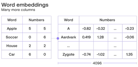
For more information on embeddings and how they work, I recommend starting with Cohere’s What Are Word and Sentence Embeddings? .
Choosing the correct size for the vocabulary embeddings is important, both for downstream performance and computational efficiency. There’s a potential tradeoff when increasing the model’s vocabulary size between training difficulty due to more tokensI discuss this training problem in more detail in the weight tying section., and representational ease due to compressing more information into a fixed number of tokens. In CrammingJonas Geiping and Tom Goldstein. 2022. Cramming: Training a Language Model on a Single GPU in One Day. arXiv:2212.14034., Geiping and Goldstein found that increasing BERT’s vocabulary size improves downstream performance until it plateaus at BERT’s original vocabulary size of 32,768 tokens.
For computational efficiency, Andrej Karpathy found that increasing nanoGPT’s vocabulary size from 50,257 to 50,30450,304 is the nearest power of 2 and multiple of 64. led to a ~25 percent increase in training speedTo be clear, this is training speed for the entire model, not just the embedding layers.. On larger models, the speedup is slower but still substantial. For training efficiency on the most accelerators, choosing a power of 2 and multiple of 8, 64, and/or 128 is important for the hardware tiling which provides the speedup and sharding across multiple accelerators.
PyTorch implements its embeddings as a lookup table of shape input_dimension, embedding_ _dimension. Each row contains an embedding vector for a specific input token. The output vector of the embedding layer is the token vector which is passed through the model’s Transformer layers.
To define the vocabulary embedding, pass in the vocabulary size and the embedding size to nn.Embedding.
# embeddings of shape vocabulary size, embedding size (C)
# input shape (B, S), output shape (B, S, C)
vocab_embed = nn.Embedding(vocab_size, hidden_size)
# Positional Encodings & Embeddings
Outside of causal masking, the Attention mechanism treats all token positions equally. Meaning the Transformer has no inherent notion of token order, as all tokens are processed simultaneously in parallelThe Feed Forward operates on each token independently of all other tokens in the sequence, so Attention is the only operation which could consider token position.. Almost all Transformers rectify this by adding positional embedding or positional encoding vectors to their token embedding vectorsAlthough implementation details can vary greatly between models..
The original Transformer in Attention Is All You Need used sinusoidal positional encodings. These positional encodings are fixed, and defined by the following formula
where is the token position in the sequence, is the model dimensionality, i.e. embedding or hidden size, and is the index from in the positional encoding vector.
PositionalEncoding is based on code from TorchText and Jonas Geiping’s crammingThis results in a unique encoding for each position in the token sequence, with tokens positionally close to each other having similar position encodingsFor more details on positional encodings, check out Transformer Architecture: The Positional Encoding and The Illustrated Transformer..
class PositionalEncoding(nn.Module):
    def __init__(self,
        context_size: int,
        hidden_size: int
    ):
        super().__init__()
        # create the positional encoding tensor of shape
        # maximum sequence length (MS) by embedding dimension (C)
        pe = torch.zeros(context_size, hidden_size, dtype=torch.float)

        # pre-populate the position and the div_terms
        position = torch.arange(context_size).unsqueeze(1)
        div_term = torch.exp(
            torch.arange(0, hidden_size, 2) * (-math.log(10000) / hidden_size)
        )

        # even positional encodings use sine, odd cosine
        pe[:, 0::2] = torch.sin(position * div_term)
        pe[:, 1::2] = torch.cos(position * div_term)

        # register as a buffer so autograd doesn't modify
        self.register_buffer('pe', pe.unsqueeze(0), persistent=False)

    def forward(self, x: Tensor):
        # return the pre-calculated positional encodings
        # up to sequence length (S). output shape (1, S, C)
        return self.pe[:, :x.shape[1], :]
Both BERT and GPT-2 use learnable positional embeddings. Unlike positional encodings which provide a fixed mapping of positions, learnable positional embeddings are randomly initialized and updated during training. This allows the model to adapt the positional vectors to fit the task and data and potentially learn more complex position relationships.
Positional embeddings are initialized the same way as vocabulary embeddings, except across maximum sequence length and the embedding, or hidden size.
# embeddings of shape max sequence length (MS) by embedding dimension (C)
pos_embed = nn.Embedding(context_size, hidden_size)
Both positional embeddings and encodings are added to the vocabulary embeddings before the combined token embedding is passed to the model’s Transformer layers.
# Weight Tying
The final layer of a Transformer is the prediction head. It converts token vectors processed by the Attention and Feed Forward layers into token predictions. These predictions are a probability distributionThese probabilities are in log space, so they are often referred to as the model’s logits. across all possible tokens in the vocabulary.
The model head is implemented as single linear layer, optionally with a preceding normalization layer. Like all linear layers in our Transformer, the bias term will be optional.
# converts input token vectors of shape (B, S, C) to probability
# distribution of shape batch, sequence length, vocabulary size (B, S, VS)
head = nn.Linear(hidden_size, vocab_size, bias=head_bias)
Since the vocabulary embedding and prediction head share the same input and output dimensions, the prediction head has the same weight shape as the vocabulary embedding. This observation led to weight tyingOfir Press and Lior Wolf. 2017. Using the Output Embedding to Improve Language Models. In Proceedings of the 15th Conference of the European Chapter of the Association for Computational Linguistics: Volume 2, Short Papers, Association for Computational Linguistics, 157–163. Retrieved from https://aclanthology.org/E17-2025Hakan Inan, Khashayar Khosravi, and Richard Socher. 2017. Tying Word Vectors and Word Classifiers: A Loss Framework for Language Modeling. arXiv:1611.01462., the practice of setting the vocabulary embedding to share the same set of weights as the prediction head. Weight tying assumes that there is enough similarity between creating token embeddings and predicting tokens for shared weights to learn a representation which completes both tasks, and in practice it works.
Weight tying has two main the benefits. First, it reduces the number of parameters in the model, leading to lower memory usage and faster computation speed. For example, PaLMAakanksha Chowdhery, Sharan Narang, Jacob Devlin, Maarten Bosma, Gaurav Mishra, Adam Roberts, Paul Barham, Hyung Won Chung, Charles Sutton, Sebastian Gehrmann, Parker Schuh, Kensen Shi, Sasha Tsvyashchenko, Joshua Maynez, Abhishek Rao, Parker Barnes, Yi Tay, Noam Shazeer, Vinodkumar Prabhakaran, Emily Reif, Nan Du, Ben Hutchinson, Reiner Pope, James Bradbury, Jacob Austin, Michael Isard, Guy Gur-Ari, Pengcheng Yin, Toju Duke, Anselm Levskaya, Sanjay Ghemawat, Sunipa Dev, Henryk Michalewski, Xavier Garcia, Vedant Misra, Kevin Robinson, Liam Fedus, Denny Zhou, Daphne Ippolito, David Luan, Hyeontaek Lim, Barret Zoph, Alexander Spiridonov, Ryan Sepassi, David Dohan, Shivani Agrawal, Mark Omernick, Andrew M. Dai, Thanumalayan Sankaranarayana Pillai, Marie Pellat, Aitor Lewkowycz, Erica Moreira, Rewon Child, Oleksandr Polozov, Katherine Lee, Zongwei Zhou, Xuezhi Wang, Brennan Saeta, Mark Diaz, Orhan Firat, Michele Catasta, Jason Wei, Kathy Meier-Hellstern, Douglas Eck, Jeff Dean, Slav Petrov, and Noah Fiedel. 2022. PaLM: Scaling Language Modeling with Pathways. arXiv:2204.02311. has a vocabulary of 256 thousand tokens and with weight tying the 540B model’s embedding layer and prediction head share ~4.7 million parametersCalculated by multiplying the number of tokens in the vocabulary by the reported of 18,432 for PaLM 540B.. Without weight tying the parameter count for both the vocabulary embedding and prediction head would double to 9.4 million.
The second benefit of weight tying is it can improve model convergence, especially for models with large vocabularies relative to the training dataset. Without weight tying, the vocabulary embedding layer only updates embeddings for tokens in the current batch, while the prediction head receives an update across the entire vocabularyEven if it’s a small update due to the prediction head correctly assigning a low probability of token selection.. Since language follows a near-Zipfain distribution, this means tokens in the long tails will have far fewer updates then tokens in the middle of the distribution. Since weight tying halves the total token parameters, the model requires less updates to learn the combined embedding. Additionally, the combined embedding will receive updates every step due to the predictions from the model head, instead of only updating when the token is used.
Weight tying does have a potentially significant downside. Since prediction and vocabulary embedding tasks are somewhat orthogonal to each otherJun Gao, Di He, Xu Tan, Tao Qin, Liwei Wang, and Tie-Yan Liu. 2019. Representation Degeneration Problem in Training Natural Language Generation Models. arXiv:1907.12009., a model trained with weight tying suffers a performance hitCharles Welch, Rada Mihalcea, and Jonathan K. Kummerfeld. 2020. Improving Low Compute Language Modeling with In-Domain Embedding Initialisation. arXiv:2009.14109. relative to a model trained without weight tyingAssuming it’s trained on enough data so infrequent token embeddings learn a good representation..
Most recent decoder-only models with smaller vocabularies chose to forgo weight tying, however there are a few notable exceptions which prefer the lower memory usage of weight tyingFor example, GPT-NeoX & Pythia, LLaMA, Falcon, and Llama 2 all forgo weight tying. While MPT and StarCoder both use weight tying..
For encoder-only models weight tying is widely used for pretrainingWith Cramming BERT and British Corpus BERT both tying embedding and prediction head weights.. The Masked Language Modeling task, where 10-15 percent of input tokens are replaced with a mask token, and only those 10-15 percent recieve predictions and updates, means untied embedding weights would have even sparser updates than decoder pretrainingIn typical decoder-only model pretraining, all tokens in a batch have predictions and thus updates.. This likely lends weight tying more importance to efficient encoder-only model training and explains why it is still common in recent encoder-only models.
Mechanically, weight tying is easy to implement, all we need to doAlthough some distributed setups may need a more careful implementation. is set the head weight to the vocab weight after the head has been defined.
if tie_weights:
    self.head.weight = self.vocab_embed.weight
If the prediction head has bias term, it will not be tied, as the embedding layer does not have a bias term.
# GPT-2
This GPT-2 implementation is based on Andrej Karpathy’s nanoGPTNow that we’ve defined all the individual components needed to define a Transformer, we’ll start by creating a GPT-2 model. As the GPT series are decoder-only, or autoregressive models, we will use the CasualAttention implementation we defined in the first post in this series.
This implementation is for training, not inference. Modifications for efficient inference and training will be the subject of a future post.
# GPT-2 Initialization
The __init__ method for GPT-2 is where we mix all the pieces of the Transformer together. We define our vocabulary and positional embeddings, with optional embedding dropout, initialize all the Transformer layers with CausalAttention, add the optional head normalization, create the language modeling head, and optionally tie the head and vocab embeddings weights.
For this implementation I chose to register the positional indices as a PyTorch buffer rather than create a new tensor on the fly every forward pass. But the difference in practice should be minimal.
class GPT2(nn.Module):
    def __init__(self,
        num_layers:int,
        vocab_size:int,
        hidden_size:int,
        num_heads:int,
        context_size:int,
        expand_size:int,
        attention:nn.Module=CausalAttention,
        act:nn.Module=nn.GELU,
        embed_drop:float=0.1,
        attn_drop:float=0.1,
        out_drop:float=0.1,
        ffn_drop:float=0.1,
        head_norm:bool=True,
        tie_weights:bool=True,
        head_bias:bool=True,
        bias:bool=True,
    ):
        # initialize vocab & positional embeddings to convert
        # numericalized tokens and position indicies to token
        # and position vectors, with optional dropout
        self.vocab_embed = nn.Embedding(vocab_size, hidden_size)
        self.pos_embed = nn.Embedding(context_size, hidden_size)
        self.embed_drop = nn.Dropout(embed_drop)

        # initialize num_layers of transformer layers
        self.tfm_blocks = nn.ModuleList([TransformerBlock(
                hidden_size=hidden_size, num_heads=num_heads,
                context_size=context_size, expand_size=expand_size,
                attention=attention, act=act, bias=bias,
                attn_drop=attn_drop, out_drop=out_drop,
                ffn_drop=ffn_drop)
            for _ in range(num_layers)])

        # optional pre-head normalization
        if head_norm:
            self.head_norm = nn.LayerNorm(hidden_size)
        else:
            self.head_norm = nn.Identity()

        # predicts the next token in the sequence
        self.head = nn.Linear(hidden_size, vocab_size, bias=head_bias)

        # optionally set the vocab embedding and prediction
        # head to share weights
        if tie_weights:
            self.head.weight = self.vocab_embed.weight

        # precreate positional indices for the positional embedding
        pos = torch.arange(0, context_size, dtype=torch.long)
        self.register_buffer('pos', pos, persistent=False)

        self.apply(self._init_weights)
To keep the initialization from being too verbose, I left out the weight initialization. You can view the full implementation in commented-transformers.
# GPT-2 Forward
The first part of GPT-2 forward method is to create both the vocabulary and positional embeddings. The positional embeddings are added to the vocabulary embeddings. Then the rest of the model is straight forward: pass the token vectors through each Transformer layer, the optional head normalization layer, and the language modeling prediction head.
def forward(self, x: Tensor):
    # convert numericalized tokens of shape (B, S)
    # into token embeddings of shape (B, S, C)
    tokens = self.vocab_embed(x)
    pos = self.pos_embed(self.pos[:x.shape[1]])

    # positional embeddings are added to token embeddings
    x = self.embed_drop(tokens + pos)

    # pass token vectors through all transformer layers
    for block in self.tfm_blocks:
        x = block(x)

    # apply optional pre-head normalization
    x = self.head_norm(x)

    # converts input token vectors of shape (B, S, C) to
    # probability distribution of shape batch, sequence length,
    # vocabulary size (B, S, VS)
    return self.head(x)
And there you have it. Our first fully defined Transformer model. You can view the full implementation in commented-transformers..
# Causal Language Modeling
For simplicity, I decided not to add a loss calculation in the forward method of the base GPT-2 model. However, since the most popular Transformers libraryThat would be Hugging Face’s Transformers. uses this method, we will implement it. Remember that a causal language model’s objective is to predict the next token from the current token. If we used the first sentence in this post and assume each word is a token:
Transformers are everywhere.
then the “Transformers” token would predict “are”, and “are” would predict “everywhere.”
To create our inputs (line 1) we’ll drop the last token, and to create the labels (line 2) we’ll remove the first token:
- Transformers are
- are everywhere.
Since each token is predicting one token, we’ll use Cross Entropy as the loss function. nn.CrossEntropyLoss expects the prediction shape to be , where is the number of predictions and is the number of classes, so we’ll reshape the input to match. Likewise, it expects the targets to be shape , so we’ll flatten the labels into one dimension.
class GPT2ForCausalLM(GPT2):
    def __init__(self,
        loss_fn:nn.Module=nn.CrossEntropyLoss(),
        **kwargs
    ):
        super().__init__(**kwargs)
        self.loss_fn = loss_fn

    def forward(self, x: Tensor):
        # the labels are the next token, so remove the first token
        # & resize inputs to same length as labels by dropping last token
        inputs = x[:, :-1]
        labels = x[:, 1:]

        # logits are of shape batch, sequence length, vocab size (B, S, VS),
        # labels are of shape batch, vocab size (B, S)
        logits = super().forward(inputs)

        # flatten logits into (B*S, VS) and labels into (B*S) & calculate loss
        loss = self.loss_fn(logits.view(-1, logits.shape[-1]), labels.view(-1))

        # return both the logits and the loss
        return {'logits': logits, 'loss': loss}
Now our GPT-2 model is trainable. You can view the full implementation in commented-transformers..
# BERT
The BERT implementation is inspired by Jonas Geiping’s cramming along with Andrej Karpathy’s nanoGPT.The second model we’ll define is BERT. BERT is a encoder-only model, which means we need to use the BidirectionalAttention implementation we defined in the first post in this series.
Modern encoder-only models are trained on the Masked Language Modeling taskHistorically, BERT models also used Next Sentence Prediction in combination with Masked Language Modeling. But starting with RoBERTa, this task was dropped., where 10-15 percent of input tokens are replaced with a mask token, and the model has to predict the masked token.
- “MASK are everywhere.”
- “Transformers are everywhere.”
# BERT Initialization
Our BERT initialization is almost identical to GPT-2, except for two changes. First, as mentioned earlier we use Bidirectional Attention instead of Causal. Second, following Cramming BERT, I switched out the original BERT’s learned positional embeddings for fixed positional encodings. Everything else remains the same as our GPT-2 implementation.
class BERT(nn.Module)
    def __init__(self,
        # rest of args are the same as GPT-2 __init__
        attention:nn.Module=BidirectionalAttention,
        ...
    ):
        self.vocab_embed = nn.Embedding(vocab_size, hidden_size)
        # swap out positional embeddings for encodings
        self.pos_encode = PositionalEncoding(context_size, hidden_size)
        self.embed_drop = nn.Dropout(embed_drop)

        self.tfm_blocks = nn.ModuleList([TransformerBlock(
                hidden_size=hidden_size, num_heads=num_heads,
                context_size=context_size, expand_size=expand_size,
                attention=attention, act=act, bias=bias,
                attn_drop=attn_drop, out_drop=out_drop,
                ffn_drop=ffn_drop)
            for _ in range(num_layers)])

        if head_norm:
            self.head_norm = nn.LayerNorm(hidden_size)
        else:
            self.head_norm = nn.Identity()

        self.head = nn.Linear(hidden_size, vocab_size, bias=head_bias)

        if tie_weights:
            self.head.weight = self.vocab_embed.weight

        self.apply(self._init_weights)
# BERT Forward
Most of the BERT changes are in the forward method. Here I am skipping the basic BERT forward and jumping stright to a combined BERTForMaskedLM for pretraining forward, which has support for the Masked Label Modeling task. The labels only exist for the masked tokens, with all the other tokens replaced with Cross Entropy Loss’s ignore_index in the DataLoader. So we can save a bit of compute by only selecting the masked tokens for prediction and loss calculation.
class BERTForMaskedLM(BERT):
    def __init__(self,
        loss_fn:nn.Module=nn.CrossEntropyLoss(),
        **kwargs
    ):
        super().__init__(**kwargs)
        self.loss_fn = loss_fn

    def forward(self, x: Tensor, labels: Tensor):
        # convert numericalized tokens of shape (B, S)
        # into token embeddings of shape (B, S, C)
        tokens = self.vocab_embed(x)
        pos = self.pos_encode(self.pos[:x.shape[1]])

        # positional encodings are added to token embeddings
        x = self.embed_drop(tokens + pos)

        # pass token vectors through all transformer layers
        for block in self.tfm_blocks:
            x = block(x)

        # apply optional pre-head normalization
        x = self.head_norm(x)

        # only select the masked tokens for predictions
        # reshapes x to (B*S, VS) and labels to (B*S)
        mask_tokens = labels != self.loss_fn.ignore_index
        x = x[mask_tokens]
        labels = labels[mask_tokens]

        # converts input token vectors of shape (B*S, C)
        # to probability distribution of shape (B*S, VS)
        logits = self.head(x)

        # return both the logits and the loss
        return {'logits': logits, 'loss': self.loss_fn(logits, labels)}
And there we have it, a modern BERT encoder-only model. The full implementation in commented-transformers has been split into BERT and BERTForMaskedLM, with the latter’s forward method modified to support indexing using torch.compile with fullgraph=True.
# Conclusion
Between this post and the previous post on Attention, I have shown you how to implement an entire Transformer model, ultimately creating two both a decoder model and encoder model: GPT-2 and BERT. You should now be able to write your own Transformer and have the foundation to follow model-specific modifications to the Transformer architecture.
In future posts I will cover some standard modifications to the basic Transformer architecture and how to implement faster training and inference.