Tinkering With Attention Pooling

Improving Upon Learned Aggregation

Benjamin Warner

July 14, 2022

23 min. read

Almost all modern convolutional neural networks (CNNs), use Global Average PoolingMin Lin, Qiang Chen, and Shuicheng Yan. 2013. Network In Network. arXiv:1312.4400. to transform the results image dimensions $(N,C,H,W)$The dimensions $(N,C,H,W)$ are batch, channel, height, and width, respectively. to reduce to $(N,C)$ before making the final class predictions.

The primary exception in vision neural networks comes from Transformer based networks, which depending on the architecture can use pooling or the results straight from the Transformer.

Last year, there were at least three papers which proposed variations on Attention Pooling for use with CNNs. The first paper I noticed was Touvron et al’sHugo Touvron, Matthieu Cord, Alaaeldin El-Nouby, Piotr Bojanowski, Armand Joulin, Gabriel Synnaeve, and Hervé Jégou. 2021. Augmenting Convolutional networks with attention-based aggregation. arXiv:2112.13692. Augmenting Convolutional networks with attention-based aggregation, who propose Learned Aggregation, their flavor of resolution independent Attention Pooling, and create a new CNN architecture to specifically take advantage of itThe other two papers are the CNN half of CLIP in Learning Transferable Visual Models From Natural Language Supervision and a zero-shot capable Attention Pooling mechanism in ML-Decoder: Scalable and Versatile Classification Head..

In this post, I explain what Attention Pooling is and how it works using Touvron et al’s Learned Aggregation as an example. I experiment with Learned Aggregation using XResNeXt—the fastai version of ResNeXtSaining Xie, Ross Girshick, Piotr Dollar, Zhuowen Tu, and Kaiming He. 2017. Aggregated Residual Transformations for Deep Neural Networks. In Proceedings of the IEEE Conference on Computer Vision and Pattern Recognition (CVPR).—on several small datasets. I modestly improve upon Learned Aggregation’s results with some small architectural tweaks. I also report results from my experiments with hybrid pooling layers that combine Average and Attention Pooling which outperform Learned Aggregation in the small dataset regime.

My best performing hybrid layer, Concat Attention Pooling which concatenates the output of Average Pooling with a modified Learned Aggregation, outperforms Learned Aggregation with an F1 Score improvement of 0.06 for Kaggle Petals, and an improvement in accuracy of 0.99 percentage points on Imagenette and 2.98 percentage points on ImageWoof.

However, all these results lagAlthough the gap is close for one dataset. behind the performance of Average Pooling. This result suggests that Learned Aggregation-style Attention Pooling and layers derived from it are still mostly inferior in the small dataset regime.

# Quick Recap of Attention

If you are unfamiliar with Attention in a neural network context, you should pause and read Attention Is All You Need by Vaswani et alAshish Vaswani, Noam Shazeer, Niki Parmar, Jakob Uszkoreit, Llion Jones, Aidan N. Gomez, Lukasz Kaiser, and Illia Polosukhin. 2017. Attention is All You Need. In Proceedings of the 31st International Conference on Neural Information Processing Systems (NIPS’17), 6000–6010. or one of the many good Transformer summaries. Personally, I recommend Jay Alammar’s The Illustrated Transformer.

A quick recap of Attention in Transformers. 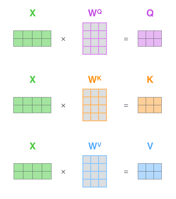Query, key, and value calculation in matrix form. From The Illustrated Transformer.Attention works by creating query $Q$, key $K$, and value $V$ matrices from inputs $X$ via linear layers with learnable weights $W^Q$, $W^K$, and $W^V$.

$$Q=XW^Q \newline K=XW^K \newline V=XW^V$$

self-attention is then calculated by:

$$\tag{1}\mathrm{Attention}(Q, K, V) = \mathrm{softmax}\left(\frac{QK^T}{\sqrt{d_k}}\right)V$$

where $\sqrt{d_k}$ is a scaling factor, usually based on the number of heads in the case of multi-headed attention.

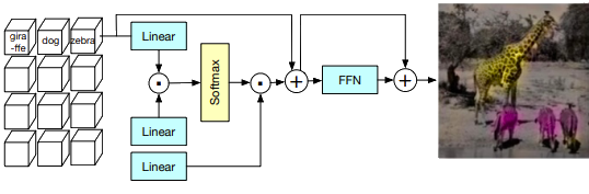
This process is illustrated by Jay Alammar in Figure 1 on the rightFigure 1 is above if reading on mobile. and Figure 2 below.

Self-attention calculation in matrix form with attention denoted as $Z$. From The Illustrated Transformer.

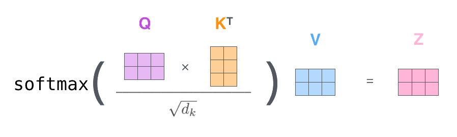
The resulting $\mathrm{Attention}(Q, K, V)$ is usually passed through projection linear layer and a feed forward network (FFN) before finishing the attention block.

This overall procedure is the same in most Transformer implementations, with differences in normalization, positional embeddingsOf which there are many flavors and variations. or lack-thereof, softmax substitutes for calculating self-attention, or modifications to calculate Attention & FFN concurrently.

# Attention Pooling

Attention Pooling uses the same self-attention process with one significant modification. In a normal implementation, the output of the attention mechanism is the same dimension as the input $X$. But when pooling, the batch image dimensions $(B,C,H,W)$Vision Transformers usually transform the image dimensions $(N,C,H,W)$ to $(N,HW,C)$ for calculating attention, or create patch vectors from the images. need to be reduced to $(N,C)$, so they can be passed through the one dimensional linear final layer(s).

The allure of using Attention Pooling over Average or Max Pooling is Attention Pooling could use the self-attention mechanism pick the best set of two-dimensional features to transform into one-dimensional features for the final classification layer, unlike Average or Max Pooling which squashIn practice, the model is trained to provide information which will survive the mean or max operation. the two-dimensional information into one dimension.

# Learned Aggregation

Learned Aggregation is one implementation of Attention Pooling by Touvron et al. It behaves like a normal self-attention mechanism with a few adjustments to transform Attention into a learnable pooling mechanism.

Using the same notation as above, Learned Aggregation removes the input $X$ as the basis for the query and replaces it with a learnable fixed vector $q_{\mathrm{cls}}$ to create a class query $Q_{\mathrm{cls}}$ using the query linear layer $W^Q$.

$$Q_{\mathrm{cls}}=q_{\mathrm{cls}}W^Q$$

From there, the self-attention mechanism behaves as normal, with $Q_{\mathrm{cls}}$ being the only difference from Equation 1:

$$\tag{2} \mathrm{Attention_{cls}}(Q_{\mathrm{cls}}, K, V) = \mathrm{softmax}(\frac{Q_{\mathrm{cls}}K^T}{\sqrt{d_k}})V$$

Since this fixed vector class input $q_{\mathrm{cls}}$ is defined to be size $(1, C)$Ignoring broadcasting., this means the result of the matrix multiplication in the attention mechanism will be $(N,C)$ as desiredThe paper also introduces an attention map per class by replacing the class vector $q$ with a class matrix $Q$ of size $(n, C)$, where $n$ is the number of classes. This requries $n$ final linear layers, one per class..

The class vector $q_{\mathrm{cls}}$ is added to $\mathrm{Attention_{cls}}$ as a residual before the feed forward network, before passing the entire Learned Aggregation results to the final linear layer.

Learned Aggregation, with the input $X$ from the CNN and final linear layer hidden.

Of significant note, the source code for PatchConvNet contains an important feature unspecified in the paper—a per channel learnable $\gamma$ adjustments applied to the attention and FFN output.

A clean implementation of Learned Aggregation can be found in the Implementation Appendix.

# Tinkering With Attention Pooling

⊕Code and training logs for this post are available here.Touvron et al. developed a new CNN architecture, PatchConvNet, specifically designed to benefit attention pooling,

We need an architecture producing a higher-resolution feature maps in order to better leverage the proposed attention-based pooling.

However, they also mention that Learned Aggregation improves a ResNet Strikes BackRoss Wightman, Hugo Touvron, and Hervé Jégou. 2021. ResNet strikes back: An improved training procedure in timm. arXiv:2110.00476. ResNet50Kaiming He, Xiangyu Zhang, Shaoqing Ren, and Jian Sun. 2016. Deep Residual Learning for Image Recognition. In Proceedings of the IEEE Conference on Computer Vision and Pattern Recognition (CVPR). on Imagenet:

Our Learned Aggregation stage increases the performance of a very competitive ResNet model. When adopting the recent training recipe from Wightman et al., we obtain 80.1% top-1 accuracy on Imagenet1k by adding a learned pooling to a ResNet50. This is an improvement of +0.3%.

Since PatchConvNet-S60S60 is the smallest proposed version of PatchConvNet in Touvron et al. is just under two times slower compared to a XResNeXt50Most of the slowdown is probably due to PyTorch not having an efficient LayerNorm implementation for BCHW tensors., and the speed penalty increases further when compared to a plain ResNet, I will focus on testing how Learned Aggregation, and Attention Pooling in general, might improve a ResNet based architecture.

# Base Model

For my experiments, I use XResNeXt50—the fastai version of ResNeXt with architectural improvements from the Bag of TricksTong He, Zhi Zhang, Hang Zhang, Zhongyue Zhang, Junyuan Xie, and Mu Li. 2019. Bag of Tricks for Image Classification with Convolutional Neural Networks. In 2019 IEEE/CVF Conference on Computer Vision and Pattern Recognition (CVPR), 558–567. DOI:10.1109/CVPR.2019.00065 paper—with the Efficient Channel AttentionQilong Wang, Banggu Wu, Pengfei Zhu, Peihua Li, Wangmeng Zuo, and Qinghua Hu. 2019. ECA-Net: Efficient Channel Attention for Deep Convolutional Neural Networks. arXiv:1910.03151. module, replacing all stem and body activation functions with the MishDiganta Misra. 2019. Mish: A self regularized non-monotonic neural activation function. arXiv:1908.08681. activation function, and replacing the stem pooling layers with MaxBlurPoolRichard Zhang. 2019. Making Convolutional Networks Shift-Invariant Again. arXiv:1904.11486. and ResBlock pooling layers with BlurPool.

Furthermore, since Touvron et al. mention Learned Aggregation works best with a wider input resolution, I tested a modification to XResNeXt50 which increased Attention Pooling performance. XResNeXt50S skips the last downsample and increase from 1024 to 2048 channels while still retaining the same total number of ResBlock layers $[3,4,9]$ as XResNext50 $[3,4,6,3]$.

In the small dataset regime, XResNeXt50S is competitive with, and sometimes outperforms, XResNeXt50 even when using the default average pooling layer.

# Training Setup

All models were trained with mixed precision for 80 epochs on a batch size of 64, using the RangerLess Wright. 2019. New Deep Learning Optimizer, Ranger: Synergistic combination of RAdam LookAhead for the best of both. (August 2019). Retrieved from https://lessw.medium.com/new-deep-learning-optimizer-ranger-synergistic-combination-of-radam-lookahead-for-the-best-of-2dc83f79a48d optimizer with a flat learning rate followed by cosine decay starting at seventy-five percent of total training steps. All other settings used fastai’s defaults.

All models were trained with random crops and each batch used MixUpHongyi Zhang, Moustapha Cisse, Yann N. Dauphin, and David Lopez-Paz. 2017. mixup: Beyond Empirical Risk Minimization. arXiv:1710.09412., CutMixSangdoo Yun, Dongyoon Han, Seong Joon Oh, Sanghyuk Chun, Junsuk Choe, and Youngjoon Yoo. 2019. CutMix: Regularization Strategy to Train Strong Classifiers with Localizable Features. arXiv:1905.04899., or additional augmentationUsing the CutMixUpAugment callback from my fastxtend package.. The additional augmentation included warping, rotation, flipping, and lighting and color changes.

Augmentation details for each dataset can be seen in the Dataset Appendix.

Each model was trained for 15,920 steps on Kaggle Petals, 11,760 steps on Imagenette, and 11,280 steps on ImageWoof.

All reported results are the mean of three training runs, each with a different seed of $42$​​​​​​, $\phi$​​​​​​, $\pi$.

# Baseline Results

Table 1 below shows baseline results from training a XResNeXt50 and XResNeXt50S with Average Pooling and XResNeXt50S with Learned Aggregation.

Baseline Results

			Accuracy		F1 Score		Matthews Coefficient		Train Loss		Valid Loss
Dataset	Model	Learning Rate	Mean	St. Dev	Mean	St. Dev	Mean	St. Dev	Mean	St. Dev	Mean	St. Dev
Kaggle Petals	XResNeXt50	8e-3	91.10%	0.23%	0.9212	0.0014	0.9238	0.0013	1.3028	0.0281	1.0858	0.0048
	XResNeXt50S	8e-3	90.66%	0.19%	0.9179	0.0014	0.9227	0.0008	1.2990	0.0275	1.1014	0.0014
	Learned Aggregation	6e-4	85.10%	0.29%	0.8602	0.0022	0.8707	0.0017	1.4923	0.0348	1.2578	0.0011
Imagenette	XResNeXt50	8e-3	95.53%	0.19%			0.9504	0.0021	0.8314	0.0115	0.6265	0.0065
	XResNeXt50S	8e-3	95.80%	0.11%			0.9533	0.0012	0.8261	0.0134	0.6240	0.0053
	XResNeXt50S	2e-3	94.96%	0.23%			0.9440	0.0025	0.8368	0.0137	0.6473	0.0063
	Learned Aggregation	2e-3	94.36%	0.16%			0.9374	0.0018	0.8432	0.0152	0.6555	0.0154
ImageWoof	XResNeXt50	8e-3	90.78%	0.17%			0.8974	0.0019	0.9068	0.0252	0.7660	0.0083
	XResNeXt50S	8e-3	90.47%	0.11%			0.8940	0.0013	0.9172	0.0270	0.7671	0.0069
	Learned Aggregation	9e-4	87.14%	0.29%			0.8568	0.0032	0.9767	0.0303	0.8372	0.0053

All results are from a mean of three seeded runs. For Kaggle Petals, Accuracy is Balanced Accuracy. All models are the XECA-XResNeXt50 architecture. Learned Aggregation has a XECA-XResNeXt50S body.

Three things to note from the baselines.

First, XResNeXt50S can be competitive with XResNeXt50, especially on easier datasets like Imagenette, but falls short on the two tougher datasets. In the ablations I ran on ImagenetteAlthough I did not run ablations on other datasets, which is a weakness in these results., a XECA-XResNeXt50S with Learned Aggregation outperformed a XECA-XResNeXt50 with Learned Aggregation, matching Touvron et al.’s results of Learned Aggregation performing better with a wider input resolution.

Second, Learned Aggregation is more sensitive to the learning rate than Average Pooling. Average Pooling can use the same high learning rate of $8e^{-3}$ across all three datasets, while Learned Aggregation requires lowering the learning rate for both ImageWoof and Kaggle Petals. Using the same learning rate on all datasets with Learned Aggregation results in diverging training results on at least one of the three training runsFor Kaggle Petals, increasing the learning rate to $7e^{-4}$ resulted in the last of three training results to consistently diverge, indicating the learning rate isn’t stable across all training seeds..

Third, Learned Aggregation requires a lower learning rate compared to Average Pooling. And even when the learning rate is the same, $2e^{-3}$ for Imagenette, Learned Aggregation performs over half a percentage point worse in accuracy than Average Pooling. Well outside the standard deviation.

This first pass at using Learned Aggregation fails to replicate the paper’s results of similar performance on a ResNet architecture, albeit on small datasets.

# Adding NormFormer’s Sandwich Norm

Given the less than stellar results of Learned Aggregation on small datasets, I started to wonder if it would be possible to modify it to improve performance.

Inspired by the EleutherAI research community, I tried the simple change of adding Sandwich NormSandwich Norm being the EleutherAI term of art used for NormFormer-style normalization. from NormFormer: Improved Transformer Pretraining with Extra NormalizationSam Shleifer, Jason Weston, and Myle Ott. 2021. NormFormer: Improved Transformer Pretraining with Extra Normalization. arXiv:2110.09456. to Learned Aggregation.

As shown in Figure 4, Sandwich Norm adds two normalization layers to the TransformerKatherine Crowson does not recommend using Sandwich Norm in CNN ResNet style blocks, reporting worse accuracy. Only for Transformers.. One right after attention and the second after the activation function in the feed forward network.

Sandwich Norm from NormFormer.

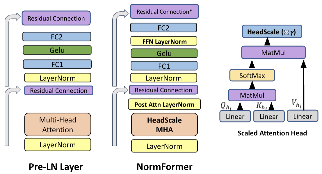
With only one Transformer module in the XECA-XResNeXt50S with Learned Aggregation, adding two more normalization layers should have a negligible result on training speed and memory usage.

The code for Learned Aggregation with Sandwich Norm can be found in the Implementation Appendix.

Learned Aggregation with Sandwich Norm

			Accuracy		F1 Score		Matthews Coefficient		Train Loss		Valid Loss
Dataset	Model	Learning Rate	Mean	St. Dev	Mean	St. Dev	Mean	St. Dev	Mean	St. Dev	Mean	St. Dev
Kaggle Petals	Learned Aggregation	6e-4	85.10%	0.29%	0.8602	0.0022	0.8707	0.0017	1.4923	0.0348	1.2578	0.0011
	Learned Sandwich	1e-3	86.84%	0.29%	0.8743	0.0033	0.8835	0.0014	1.4457	0.0387	1.2094	0.0094
Imagenette	XResNeXt50S	2e-3	94.96%	0.23%			0.9440	0.0025	0.8368	0.0137	0.6473	0.0063
	Learned Aggregation	2e-3	94.36%	0.16%			0.9374	0.0018	0.8432	0.0152	0.6555	0.0154
	Learned Sandwich	2e-3	94.62%	0.30%			0.9403	0.0033	0.8432	0.0152	0.6555	0.0154
ImageWoof	XResNeXt50S	2e-3	89.88%	0.02%			0.8874	0.0003	0.9119	0.0209	0.7794	0.0020
	Learned Aggregation	9e-4	87.14%	0.29%			0.8568	0.0032	0.9767	0.0303	0.8372	0.0053
	Learned Sandwich	1e-3	87.67%	0.08%			0.8628	0.0009	0.9705	0.0315	0.8294	0.0084

All results are from a mean of three runs. For Kaggle Petals, Accuracy is Balanced Accuracy. All models are the XECA-XResNeXt50 architecture. Learned Aggregation has a XECA-XResNeXt50S body.

Table 2 above shows the results when training Learned Aggregation with Sandwich Norm and there are some notable improvements.

Sandwich Norm allows Learned Aggregation to train with more consistent and higher learning rates. Adding it allowed an increase in Kaggle Petals’ learning rate from $6e^{-4}$ to $1e^{-3}$ and ImageWoof’s from $9e^{-4}$ to $1e^{-3}$.

This coincides with a 1.64 percent improvement in F1 Score for Kaggle Petals, increasing from 0.8602 to 0.8743, and a more modest improvement on ImagenetteWhen compared to a Average Pooling XResNeXtS trained at the same learning rate Learned Aggregation Sandwich is almost within a standard deviation of accuracy on Imagenette. and ImageWoof, the latter outside the standard deviation.

This result bolsters the EleutherAI general recommendation to add Sandwich Norm to all Transformers. Unless specified otherwise, I will use Sandwich Norm on all the Learned Aggregation derivatives moving forward.

However, even with the addition of Sandwhich Norm, Learned Aggregation still lags Average Pooling as a pooling method.

# Attention Pooling and Average Pooling

Unlike Touvron et al. who report similar and slightly better results with a Learned Aggregation ResNet50 on ImageNet, my experiments with Learned Aggregation XECA-XResNeXt50S had poor performance relative to Average Pooling. Albeit on much smaller datasetsUnfortunately, testing on larger datasets is not possible for me for a reasonable amount of time or cost..

An obvious follow-up question to these results is, can combining Attention Pooling with Average Pooling alleviate some of the shortcomings with Learned Aggregation in the small data domain? Or perhaps could a combination of the two pooling methods provide results greater than the sum of the parts?

In the next two sections I recount two of the more successful methods I tried for combining Average Pooling and Attention Pooling using Learned Aggregation as my starting point.

# Average Attention Pooling

Due to the shape mismatch, Learned Aggregation uses the learnable class query $q_{\mathrm{cls}}$ as a residual in place of the input in a standard Transformer.

In Average Attention Pooling, I replace the residual $q_{\mathrm{cls}}$ with a residual from the input, using average pooling to squash the information from two dimensions to a single dimension. I use a modeified version of Sandwich Norm, adding Average Pooling and Attention Pooling results together before one normalization.

Slim Average Attention Pooling performs the same operation but removes the feed forward network section of the Transformer and replaces it with an additional activation. Leaving an Average Pool combined with the Attention Pooling’s attention mechanism.

I also removed the per-channel learnable $\gamma$ weights in both specifications, as I found they did not consistently improve performance.

Code for both variations of Average Attention Pooling can be found in the Implementation Appendix.

Average Attention Pooling

			Accuracy		F1 Score		Matthews Coefficient		Train Loss		Valid Loss
Dataset	Model	Learning Rate	Mean	St. Dev	Mean	St. Dev	Mean	St. Dev	Mean	St. Dev	Mean	St. Dev
Kaggle Petals	XResNeXt50	8e-3	91.10%	0.23%	0.9212	0.0014	0.9238	0.0013	1.3028	0.0281	1.0858	0.0048
	XResNeXt50S	8e-3	90.66%	0.19%	0.9179	0.0014	0.9227	0.0008	1.2990	0.0275	1.1014	0.0014
	Learned Aggregation	6e-4	85.10%	0.29%	0.8602	0.0022	0.8707	0.0017	1.4923	0.0348	1.2578	0.0011
	Slim Average Attention	3e-3	89.82%	0.13%	0.9060	0.0024	0.9140	0.0012	1.3618	0.0334	1.1133	0.0078
	Average Attention	3e-3	88.15%	0.29%	0.8872	0.0025	0.9004	0.0016	1.4767	0.0389	1.1501	0.0084
Imagenette	XResNeXt50	8e-3	95.53%	0.19%			0.9504	0.0021	0.8314	0.0115	0.6265	0.0065
	XResNeXt50S	8e-3	95.80%	0.11%			0.9533	0.0012	0.8261	0.0134	0.6240	0.0053
	XResNeXt50S	4e-3	95.77%	0.10%			0.9530	0.0011	0.8249	0.0135	0.6268	0.0074
	Learned Aggregation	2e-3	94.36%	0.16%			0.9374	0.0018	0.8432	0.0152	0.6555	0.0154
	Slim Average Attention	4e-3	95.29%	0.25%			0.9476	0.0027	0.8368	0.0124	0.6273	0.0017
	Average Attention	3e-3	95.16%	0.15%			0.9462	0.0017	0.8399	0.0128	0.6309	0.0058
ImageWoof	XResNeXt50	8e-3	90.78%	0.17%			0.8974	0.0019	0.9068	0.0252	0.766	0.0083
	XResNeXt50S	8e-3	90.47%	0.11%			0.8940	0.0013	0.9172	0.027	0.7671	0.0069
	XResNeXt50S	4e-3	90.38%	0.29%			0.8929	0.0033	0.9044	0.0231	0.7695	0.0066
	Learned Aggregation	9e-4	87.14%	0.29%			0.8568	0.0032	0.9767	0.0303	0.8372	0.0053
	Slim Average Attention	2e-3	89.47%	0.08%			0.8828	0.0009	0.9358	0.0240	0.7791	0.0044
	Average Attention	1e-3	87.58%	0.20%			0.8618	0.0022	0.9687	0.0303	0.8222	0.0093

All results are from a mean of three runs. For Kaggle Petals, Accuracy is Balanced Accuracy. All models are the XECA-XResNeXt50 architecture. Unless specified, all models have a XECA-XResNeXt50S body.

Adding Average Pooling to Attention Pooling results in improved performance on these small datasets across the board. These improvements are in a large part due to allowing the models to train at a higher learning rate than Learned Aggregation with Sandwich Norm.

Despite these improvements from adding Attention Pooling as a residual connection to Attention Pooling, both flavors of Average Attention Pooling still lag plain Average Pooling, even in the Imagenette case with the same learning rate of $4e^{-3}$ for both Slim Average Attention and Average Pooling.

Slim Average Attention Pooling, which removes the Feed Forward Network from a Transformer, consistently outperforms Average Attention Pooling. This is an interesting result as it is yet another piece of evidence for Attention PoolingAt least for Learned Aggregation derived Attention Pooling. dragging down the model performance.

Both variants of Average Attention Pooling do, however, outperform Learned Aggregation. Showing that replacing the $q_{\mathrm{cls}}$ residual with an Average Pooling residual connection can improve Attention Pooling performance.

# Concat Attention Pooling

A next logical step in exploring the combination of Average Pooling and Attention Pooling is to combine them as equals. Inspired by fastai’s concat pooling, which concatenates Average Pooling and Max Poolling, Concat Attention Pooling concatenates Learned Aggregation, without the per-channel learnable $\gamma$ weights, with Attention Pooling and passes the results to the final linear layer of the model.

I modify the normalization of the pooling output to be two independent linear norm layers, one for Average and Attention Pooling. The idea is the output of both should be closer to the same scale, this minimizing the final linear layer’s ability to ignore the results of Attention Pooling. This output is then fed through an activation layer before being passed to the final linear layer for class predictions.

The code definition of Concat Attention Pooling can be found in the Implementation Appendix.

Concat Attention Pooling

			Accuracy		F1 Score		Matthews Coefficient		Train Loss		Valid Loss
Dataset	Model	Learning Rate	Mean	St. Dev	Mean	St. Dev	Mean	St. Dev	Mean	St. Dev	Mean	St. Dev
Kaggle Petals	XResNeXt50	8e-3	91.10%	0.23%	0.9212	0.0014	0.9238	0.0013	1.3028	0.0281	1.0858	0.0048
	XResNeXt50S	8e-3	90.66%	0.19%	0.9179	0.0014	0.9227	0.0008	1.2990	0.0275	1.1014	0.0014
	Learned Aggregation	6e-4	85.10%	0.29%	0.8602	0.0022	0.8707	0.0017	1.4923	0.0348	1.2578	0.0011
	Concat Attention	4e-3	90.52%	0.18%	0.9138	0.0025	0.9201	0.0009	1.3360	0.0289	1.1160	0.0027
Imagenette	XResNeXt50	8e-3	95.53%	0.19%			0.9504	0.0021	0.8314	0.0115	0.6265	0.0065
	XResNeXt50S	8e-3	95.80%	0.11%			0.9533	0.0012	0.8261	0.0134	0.6240	0.0053
	XResNeXt50S	4e-3	95.77%	0.10%			0.9530	0.0011	0.8249	0.0135	0.6268	0.0074
	Concat Attention	4e-3	95.35%	0.19%			0.9483	0.0021	0.8384	0.0087	0.6337	0.0061
ImageWoof	XResNeXt50	8e-3	90.78%	0.17%			0.8974	0.0019	0.9068	0.0252	0.766	0.0083
	XResNeXt50S	8e-3	90.47%	0.11%			0.8940	0.0013	0.9172	0.027	0.7671	0.0069
	XResNeXt50S	4e-3	90.38%	0.29%			0.8929	0.0033	0.9044	0.0231	0.7695	0.0066
	Learned Aggregation	9e-4	87.14%	0.29%			0.8568	0.0032	0.9767	0.0303	0.8372	0.0053
	Concat Attention	2e-3	90.12%	0.62%			0.8900	0.0069	0.9319	0.0256	0.7804	0.0036

All results are from a mean of three runs. For Kaggle Petals, Accuracy is Balanced Accuracy. All models are the XECA-XResNeXt50 architecture. Unless specified, all models have a XECA-XResNeXt50S body.

Of the five flavors of Attention Pooling explored in this post Concat Attention Pooling performs the closest to Average Pooling, which is unsurprising as Average Pooling is a directAlbeit behind a normalization and activation layer. input into the final classification linear layer.

Despite the lower learning rate, Concat Attention Pooling is within one standard deviation of the Average Pooling XECA-XResNeXt50S results on Kaggle Petals for Balanced Accuracy, but not the primary F1 Score metric or the Average Pooling XECA-XResNeXt50 Accuracy results for Imagenette. Both of these are just outside of the standard deviation. As before, Concat Attention Pooling still falls short of Average Pooling on all other metrics.

Like both flavors of Adaptive Average Pooling, Concat Attention Pooling also improves upon the Learned Aggregation results, with an F1 Score improvement of 0.06 for Kaggle Petals, and accuracy improvement of 0.99 percentage points on Imagenette and 2.98 percentage points on ImageWoof.

# Performance on Larger Images

One benefit of convolutional neural networks is their ability to retain, or improve upon, performance on different image sizes. An impossible feat which for some vision transformers whose input size is fixed.

Learned Aggregation does not have positional embeddings which could restrict the input size, so while training the models I tested the results increasing the validation set size from 224-pixels to 256-pixels and 384-pixels. Based on techniques like FixResHugo Touvron, Andrea Vedaldi, Matthijs Douze, and Hervé Jégou. 2019. Fixing the train-test resolution discrepancy. In NeurIPS., the expectation is all models should perform at least slightly better at the moderately higher 256-pixel resolution.

Table 5 below shows the change in model performance on the new image sizes.

Change in Metrics from 224-Pixel Images

		256-Pixel Images				384-Pixel Images
Dataset	Model	Accuracy	F1 Score	Matthews	Valid Loss	Accuracy	F1 Score	Matthews	Valid Loss
Kaggle Petals	XResNeXt50	+0.50%	+0.0047	+0.0041	-0.0052	-4.11%	-0.0292	-0.0253	+0.1235
	XResNeXt50S	+0.41%	+0.0021	+0.0040	-0.0112	-3.41%	-0.0248	-0.0210	+0.0893
	Learned Aggregation	+0.14%	-0.0008	+0.0008	-0.0120	-4.92%	-0.0479	-0.0416	+0.1176
	Learned Sandwich	+0.36%	+0.0033	+0.0035	-0.0120	-4.51%	-0.0419	-0.0354	+0.1065
	Slim Average Attention	+0.94%	+0.0116	+0.0065	-0.0156	-3.10%	-0.0229	-0.0177	+0.0612
	Average Attention	+0.58%	+0.0037	+0.0050	-0.0190	-3.74%	-0.0336	-0.0238	+0.0677
	Concat Attention	+0.16%	+0.0037	+0.0034	-0.0058	-3.69%	-0.0302	-0.0247	+0.1301
Imagenette	XResNeXt50	+0.38%		+0.0042	-0.0023	-0.46%		-0.0051	+0.0265
	XResNeXt50S	+0.01%		+0.0001	-0.0014	-0.59%		-0.0065	+0.0224
	Learned Aggregation	+0.28%		+0.0013	-0.0043	-1.36%		-0.0114	+0.0384
	Learned Sandwich	-0.15%		+0.0013	+0.0012	-1.30%		-0.0102	+0.0387
	Slim Average Attention	+0.24%		+0.0026	-0.0044	-0.57%		-0.0063	+0.0208
	Average Attention	+0.10%		+0.0012	+0.0010	-1.30%		-0.0143	+0.0360
	Concat Attention	+0.03%		+0.0004	+0.0013	-0.47%		-0.0051	+0.0294
ImageWoof	XResNeXt50	+0.31%		+0.0036	-0.0101	-1.18%		-0.0130	+0.0385
	XResNeXt50S	+0.53%		+0.0060	-0.0023	-1.58%		-0.0174	+0.0640
	Learned Aggregation	+0.30%		+0.0034	-0.0070	-1.97%		-0.0218	+0.0535
	Learned Sandwich	+0.45%		+0.0051	-0.0089	-1.90%		-0.0211	+0.0474
	Slim Average Attention	+0.46%		+0.0052	-0.0066	-0.97%		-0.0107	+0.0437
	Average Attention	+0.55%		+0.0062	-0.0085	-1.37%		-0.0152	+0.0449
	Concat Attention	+0.55%		+0.0062	-0.0045	-2.00%		-0.0222	+0.0784

A higher value is better for Accuracy, F1 Score, and Matthews Coefficient. Lower is better for Valid Loss. For Kaggle Petals Accuracy is Balanced Accuracy.

With two exceptions, Learned Aggregation on Kaggle Petal’s F1 Score and Learned Aggregation with Sandwich Norm on Imagennette Accuracy, all models have at least a slight improvement in metrics at the moderately higher 256-pixel resolution. There also doesn’t appear to be a pattern for the improvement across model specifications and datasets.

384-pixels images is quite different from the training data’s 224-pixels, so it is unsurprising that without fine tuning on this larger resolution, all model specifications preforms worse across all metrics. But like the 256-pixel images, there doesn’t appear to be a pattern across model specifications and datasets.

These two results together lead me to conclude that Learned Aggregation derived Attention Pooling does not have a consistently worse penalty on differing image sizes than an Average Pooling CNN.

# A Brief Discussion of the Results

Despite Touvron et al. matching and mildly exceeding the performance of a Average Pooling ResNet50 on ImageNet, neither Learned Aggregation or any of the four other variations I explored in this post outperformed Average Pooling in this small dataset regime.

I cannot rule out that with more compute and longer training the Attention Pooling would catch up and surpass the Average Pooling XResNet models. However, I would be a bit surprised if training longer on small datasets yields more improvements with Learned Aggregation-style pooling layers relative to Average Pooling over training on a larger dataset.

There are a few positive takeaways from these resultsOutside of I find them interesting and if you read this far I expect you do too.. First, these results show that Attention Pooling without positional encoding can be expected to perform similarly to Average Pooling on different image sizes. If a flavor of Attention Pooling were found that matches Average Pooling, then a reasonable expectation would be for it to perform similarly to Average Pooling if fined tuned on different image sizes.

Second, is these results show that there are a few simple tweaks to improve Learned Aggregation-style Attention Pooling mechanisms. Including using Average Pooling as a residual connection instead of, or perhaps in addition tooI leave it as an exercise to the reader to explore using Average Pooling and the class vector $q$ as a combined residual with Attention Pooling. For now., using the $q_{\mathrm{cls}}$ as a residual.

Last, and perhaps the most universal takeaway, would be these results are yet more evidence which shows that anyone working with Transformers should try NormFormer-style Sandwich Normalization, including when applying Transformers to vision tasks.

# Appendix: Ablations

To narrow down all of my initial ideas to I ran ablations for twenty epochs, averaging three runs across ImagenetteIf I redid these ablations, I would use Kaggle Petals and not Imagenette due to the larger difference in results the latter dataset provides..

These ablations included:

• Testing different Learning Rates
• Different normalization layers: Batch Norm, RMS Norm, and Layer Norm
• Sandwich Norm and Sandwich Norm-like normalization
• Additional Activation functions at the end of the pooling layer
• Per channel, single, and no learnable $\gamma$ parameters
• Different sized initializations for $\gamma$ parameters
• Different initializations for the Attention layers
• Removing the Feed Forward Network

Altogether, this covered over ninetyIf I was awake to notice an ablation result wasn’t going anywhere, I would stop it before it finished and move to the next one. ablations.

I then tested the most useful looking subset of these ablations for the full eighty epochs on Imagenette, ImageWoof, and then Kaggle Petals. Seventeen on Imagenette, seventeen on ImageWoof, and fourteen on Kaggle PetalsIgnoring ablations which diverged due to an incorrectly set learning rate.. The decrease is due to I removing specifications on later datasets if they did not seem useful or interesting.

These forty-eight 80-epoch ablation training logs, including the specifications discussed above, can be viewed here.

# Appendix: Implementation Code

This section has minimal implementations for all model specifications. AttentionPool2d is not replicated after the Learned Aggregation if it is unchanged. To reduce clutter, I removed all the dropout and stochastic depth options, as they are mostly unused.

Unless additional code is provided, all models use LearnedAggregationHead for the head.

def LearnedAggregationHead(
    ni:int,
    n_out:int,
    norm:Callable[[int], nn.Module]=nn.LayerNorm,
    ffn_expand:int=3,
    **kwargs
):
    head = [AttentionPooling(ni, norm=norm, ffn_expand=ffn_expand, **kwargs),
            norm(ni),
            nn.Linear(ni, n_out)]
    return head

# Learned Aggregation

A clean implementation of Learned Aggregation based on the paper and official code repository. Tested to match Touvron et al’s implementation within less than one standard deviation on Imagenette.

class AttentionPool2d(nn.Module):
    "Attention for Learned Aggregation"
    def __init__(self,
        ni:int,
        bias:bool=True,
        norm:Callable[[int], nn.Module]=nn.LayerNorm
    ):
        super().__init__()
        self.norm = norm(ni)
        self.q = nn.Linear(ni, ni, bias=bias)
        self.vk = nn.Linear(ni, ni*2, bias=bias)
        self.proj = nn.Linear(ni, ni)

    def forward(self, x:Tensor, cls_q:Tensor):
        x = self.norm(x.flatten(2).transpose(1,2))
        B, N, C = x.shape

        q = self.q(cls_q.expand(B, -1, -1))
        k, v = self.vk(x).reshape(B, N, 2, C).permute(2, 0, 1, 3).chunk(2, 0)

        attn = q @ k.transpose(-2, -1)
        attn = attn.softmax(dim=-1)

        x = (attn @ v).transpose(1, 2).reshape(B, C)
        return self.proj(x)


class LearnedAggregation(nn.Module):
    "Learned Aggregation from https://arxiv.org/abs/2112.13692"
    def __init__(self,
        ni:int,
        attn_bias:bool=True,
        ffn_expand:int|float=3,
        norm:Callable[[int], nn.Module]=nn.LayerNorm,
        act_cls:Callable[[None], nn.Module]=nn.GELU,
    ):
        super().__init__()
        self.gamma_1 = nn.Parameter(1e-4 * torch.ones(ni))
        self.gamma_2 = nn.Parameter(1e-4 * torch.ones(ni))
        self.cls_q = nn.Parameter(torch.zeros(ni))
        self.attn = AttentionPool2d(ni, attn_bias, norm)
        self.norm = norm(ni)
        self.ffn = nn.Sequential(
            nn.Linear(ni, int(ni*ffn_expand)),
            act_cls(),
            nn.Linear(int(ni*ffn_expand), ni)
        )
        nn.init.trunc_normal_(self.cls_q, std=0.02)
        self.apply(self._init_weights)

    def forward(self, x:Tensor):
        x = self.cls_q + self.gamma_1 * self.attn(x, self.cls_q)
        return x + self.gamma_2 * self.ffn(self.norm(x))

    @torch.no_grad()
    def _init_weights(self, m):
        if isinstance(m, nn.Linear):
            nn.init.trunc_normal_(m.weight, std=0.02)
            if m.bias is not None:
                nn.init.constant_(m.bias, 0)

# Learned Aggregation Sandwich Norm

LearnedAggregationSandwich uses AttentionPool2d and the LearnedAggregationHead unchanged from the Learned Aggregation implementation definition.

class LearnedAggregationSandwich(nn.Module):
    "Learned Aggregation from https://arxiv.org/abs/2112.13692"
    def __init__(self,
        ni:int,
        attn_bias:bool=True,
        ffn_expand:int|float=3,
        norm:Callable[[int], nn.Module]=nn.LayerNorm,
        act_cls:Callable[[None], nn.Module]=nn.GELU,
    ):
        super().__init__()
        self.gamma_1 = nn.Parameter(1e-4 * torch.ones(ni))
        self.gamma_2 = nn.Parameter(1e-4 * torch.ones(ni))
        self.cls_q = nn.Parameter(torch.zeros([1,ni]))
        self.attn = AttentionPool2d(ni, attn_bias, norm)
        self.norm1 = norm(ni)
        self.norm2 = norm(ni)
        self.ffn = nn.Sequential(
            nn.Linear(ni, int(ni*ffn_expand)),
            act_cls(),
            norm(int(ni*ffn_expand)),
            nn.Linear(int(ni*ffn_expand), ni)
        )
        nn.init.trunc_normal_(self.cls_q, std=0.02)
        self.apply(self._init_weights)

    def forward(self, x:Tensor):
        x = self.cls_q + self.gamma_1 * self.norm1(self.attn(x, self.cls_q))
        return x + self.gamma_2 * self.ffn(self.norm2(x))

    @torch.no_grad()
    def _init_weights(self, m):
        if isinstance(m, nn.Linear):
            nn.init.trunc_normal_(m.weight, std=0.02)
            if m.bias is not None:
                nn.init.constant_(m.bias, 0)

# Average Attention Pooling

AvgAttnPooling2d uses AttentionPool2d and the LearnedAggregationHead unchanged from the Learned Aggregation implementation definition.

class AvgAttnPooling2d(nn.Module):
    def __init__(self,
        ni:int,
        attn_bias:bool=True,
        ffn_expand:int|float=3,
        norm:Callable[[int], nn.Module]=nn.LayerNorm,
        act_cls:Callable[[None], nn.Module]=nn.GELU,
    ):
        super().__init__()
        self.cls_q = nn.Parameter(torch.zeros([1,ni]))
        self.attn = AttentionPool2d(ni, attn_bias, norm)
        self.pool = nn.AdaptiveAvgPool2d(1)
        self.norm = norm(ni)
        self.ffn = nn.Sequential(
            nn.Linear(ni, int(ni*ffn_expand)),
            act_cls(),
            norm(int(ni*ffn_expand)),
            nn.Linear(int(ni*ffn_expand), ni)
        )
        nn.init.trunc_normal_(self.cls_q, std=0.02)
        self.apply(self._init_weights)

    def forward(self, x:Tensor):
        x = self.norm(self.pool(x).flatten(1) + self.attn(x, self.cls_q))
        return x + self.ffn(x)

    @torch.no_grad()
    def _init_weights(self, m):
        if isinstance(m, nn.Linear):
            nn.init.trunc_normal_(m.weight, std=0.02)
            if m.bias is not None:
                nn.init.constant_(m.bias, 0)

# Slim Average Attention Pooling

AvgAttnPooling2dS uses AttentionPool2d unchanged from the Learned Aggregation implementation definition.

class AvgAttnPooling2dS(nn.Module):
    def __init__(self,
        ni:int,
        attn_bias:bool=True,
        ffn_expand:int|float=3,
        norm:Callable[[int], nn.Module]=nn.LayerNorm,
        act_cls:Callable[[None], nn.Module]=nn.GELU,
    ):
        super().__init__()
        self.cls_q = nn.Parameter(torch.zeros([1,ni]))
        self.attn = AttentionPool2d(ni, attn_bias, norm)
        self.pool = nn.AdaptiveAvgPool2d(1)
        self.norm = norm(ni)
        self.act = act_cls()
        nn.init.trunc_normal_(self.cls_q, std=0.02)
        self.apply(self._init_weights)

    def forward(self, x:Tensor):
        return self.act(self.norm(self.pool(x).flatten(1) + self.attn(x, self.cls_q)))

    @torch.no_grad()
    def _init_weights(self, m):
        if isinstance(m, nn.Linear):
            nn.init.trunc_normal_(m.weight, std=0.02)
            if m.bias is not None:
                nn.init.constant_(m.bias, 0)


def AvgAttnPoolHead(
    ni:int,
    n_out:int,
    norm:Callable[[int], nn.Module]=nn.LayerNorm,
    ffn_expand:int=3,
    **kwargs
):
    head = [AvgAttnPooling2d(ni, norm=norm, ffn_expand=ffn_expand, **kwargs),
            nn.Linear(2*ni, n_out)]
    return head

# Concat Attention Pooling

AvgAttnConcatPooling2d uses AttentionPool2d unchanged from the Learned Aggregation implementation definition.

class AvgAttnConcatPooling2d(nn.Module):
    def __init__(self,
        ni:int,
        attn_bias:bool=True,
        ffn_expand:int|float=3,
        norm:Callable[[int], nn.Module]=nn.LayerNorm,
        act_cls:Callable[[None], nn.Module]=nn.GELU,
    ):
        super().__init__()
        self.cls_q = nn.Parameter(torch.zeros([1,ni]))
        self.attn = AttentionPool2d(ni, attn_bias, norm)
        self.norm1 = norm(ni)
        self.norm2 = norm(ni)
        self.ffn = nn.Sequential(
            nn.Linear(ni, int(ni*ffn_expand)),
            act_cls(),
            norm(int(ni*ffn_expand)),
            nn.Linear(int(ni*ffn_expand), ni)
        )
        self.norm3 = norm(ni)
        self.pool = nn.AdaptiveAvgPool2d(1)
        self.norm4 = norm(ni)
        self.act = act_cls()
        nn.init.trunc_normal_(self.cls_q, std=0.02)
        self.apply(self._init_weights)

    def forward(self, x:Tensor):
        a = self.cls_q + self.norm1(self.attn(x, self.cls_q))
        a = a + self.ffn(self.norm2(a))
        return self.act(torch.cat([self.norm4(self.pool(x).flatten(1)), self.norm3(a)], dim=1))

    @torch.no_grad()
    def _init_weights(self, m):
        if isinstance(m, nn.Linear):
            nn.init.trunc_normal_(m.weight, std=0.02)
            if m.bias is not None:
                nn.init.constant_(m.bias, 0)


def AvgAttnConcatPoolHead(
    ni:int,
    n_out:int,
    norm:Callable[[int], nn.Module]=nn.LayerNorm,
    ffn_expand:int=3,
    **kwargs
):
    head = [AvgAttnConcatPooling2d(ni, norm=norm, ffn_expand=ffn_expand, **kwargs),
            nn.Linear(2*ni, n_out)]
    return head

# XResNeXt50 vs XResNeXt50S

Using the fastai XResNeXt derived implementation from fastxtend, creating a XResNeXt50:

def xresnext50(n_out=1000, **kwargs):
    return XResNet(ResNeXtBlock, 4, [3, 4, 6, 3], n_out=n_out, **kwargs)

verses for a XResNeXt50S:

def xresnext50s(n_out=1000,  **kwargs):
    return XResNet(ResNeXtBlock, 4, [3, 4, 9], block_szs=[64, 128, 256], n_out=n_out, **kwargs)

and the final XResNeXt50S model creation with ECA added:

def xeca_resnext50s(n_out=1000,  **kwargs):
    return XResNet(ECAResNeXtBlock, 4, [3, 4, 9], block_szs=[64, 128, 256], n_out=n_out, **kwargs)

# Appendix: Datasets

All datasets use aug_transforms from fastai, with the default affine, warp, and lighting values.

All datasets are also trained with CutMixUpAugment from fastxtend, using a $1:1:1$ ratio between MixUp, CutMix, and augmentations. Augmentations are not applied if performing MixUp or CutMix.

# Imagenette

Nine augmented images from a sample Imagenette batch.

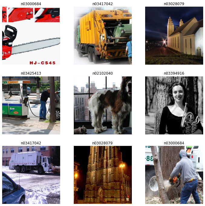
Imagenette is a subset of 10 easily classified classes from Imagenet (tench, English springer, cassette player, chain saw, church, French horn, garbage truck, gas pump, golf ball, parachute).

Imagenette is split into 9,469 training images and 3,925 validation images. Following the Imagenette leaderboard, I will evaluate model performance using accuracy.

imagenette_stats = ([0.465,0.458,0.429], [0.285,0.28,0.301])

batch_tfms = aug_transforms(max_zoom=1, max_rotate=20,
                            xtra_tfms=[Hue(), Saturation()])

DataBlock(blocks=(ImageBlock, CategoryBlock),
          splitter=GrandparentSplitter(valid_name='val'),
          get_items=get_image_files, get_y=parent_label,
          item_tfms=[RandomResizedCrop(size, min_scale=0.35), FlipItem(0.5)],
          batch_tfms=[*batch_tfms,Normalize.from_stats(*imagenette_stats)])

# ImageWoof

Nine augmented images from a sample ImageWoof batch.

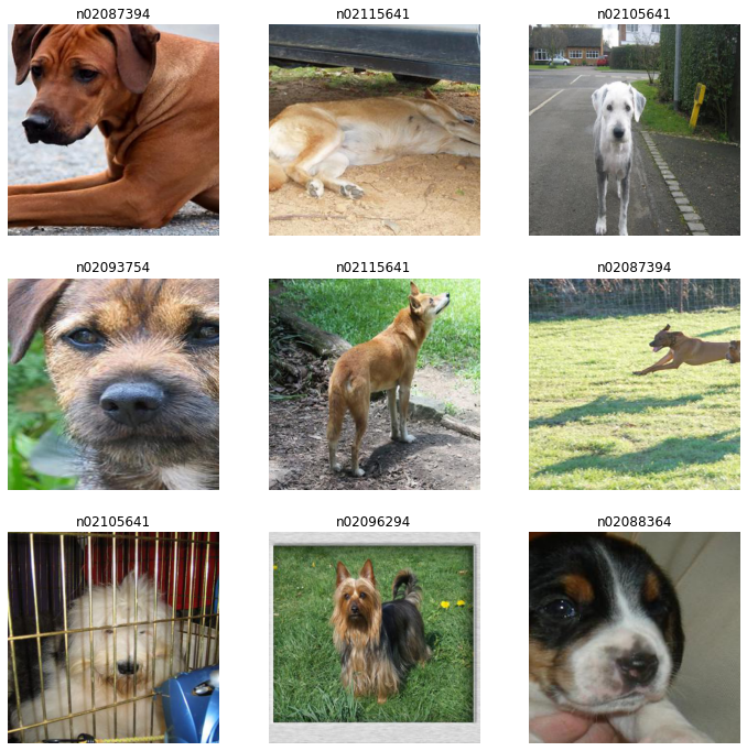
Imagewoof is a subset of 10 classes from Imagenet that aren’t so easy to classify, since they’re all dog breeds. The breeds are: Australian terrier, Border terrier, Samoyed, Beagle, Shih-Tzu, English foxhound, Rhodesian ridgeback, Dingo, Golden retriever, Old English sheepdog.

The sibling dataset to Imagenette, ImageWoof is a small fine-grained dataset. ImageWoof is split 9,025 training images and 3,929 validation images. The primary metric is also accuracy.

imagewoof_stats = ([0.496,0.461,0.399], [0.257,0.249,0.258])

batch_tfms = aug_transforms(max_zoom=1, max_rotate=20,
                            xtra_tfms=[Hue(), Saturation()])

DataBlock(blocks=(ImageBlock, CategoryBlock),
          splitter=GrandparentSplitter(valid_name='val'),
          get_items=get_image_files, get_y=parent_label,
          item_tfms=[RandomResizedCrop(size, min_scale=0.35), FlipItem(0.5)],
          batch_tfms=[*batch_tfms,Normalize.from_stats(*imagenette_stats)])

# Kaggle Petals

Nine augmented images from a sample Petals batch.The Kaggle Petals to the Metal dataset contains:

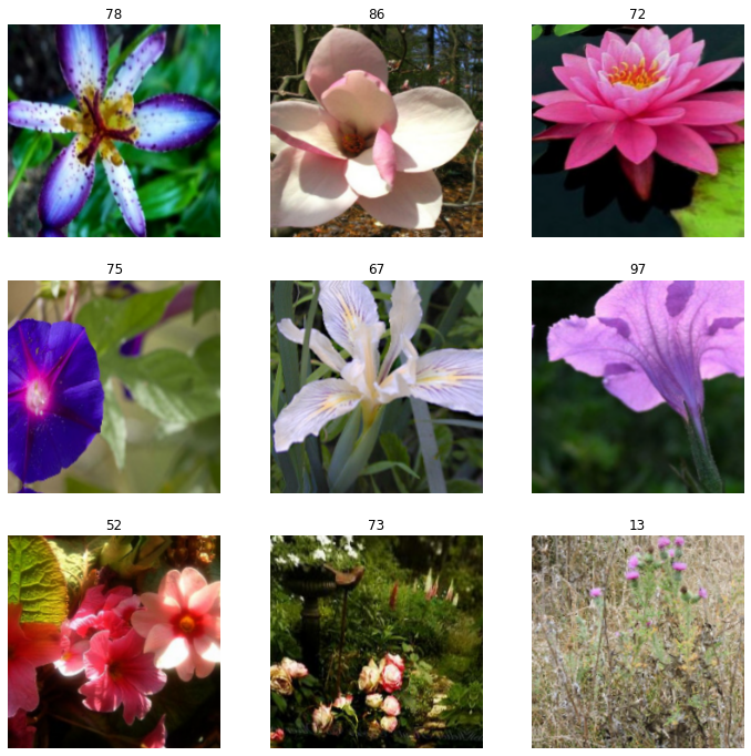
104 types of flowers based on their images drawn from five different public datasets. Some classes are very narrow, containing only a particular sub-type of flower (e.g. pink primroses) while other classes contain many sub-types (e.g. wild roses).

The dataset contains imperfections - images of flowers in odd places, or as a backdrop to modern machinery.

Petals is sourced from Kaggle. This version of the dataset was originally specified and used for the FastGarden competition in the fastai forums. The first 12,753 images are used for training and the last 3,712 images are used as the validation set. This split leads to an unequal number of classes in both the training and validation set.

Like ImageWoof, Petals to the Metal is a fine-grained classification dataset, albeit with more classes. Like the Kaggle competition the dataset originates from, I use macro F1 score for model evaluation.

petals_stats = ([0.453,0.415,0.306], [0.282,0.245,0.272])

batch_tfms = aug_transforms(ax_zoom=1, flip_vert=True, max_rotate=45,
                            xtra_tfms=[Hue(), Saturation()])

DataBlock(blocks=(ImageBlock, CategoryBlock),
          get_items=get_items,
          get_x=get_x,
          get_y=get_y,
          splitter=splitter,
          item_tfms=[RandomResizedCrop(size, min_scale=0.35)],
          batch_tfms=[*batch_tfms, Normalize.from_stats(*petals_stats)])