A few weeks ago DrivenData’s On CloudN competition finished and my solution performed decently well: finishing in the top-ten percent
In this post I will give an overview of my solution, explore some of my alternate solutions which didn’t perform as well, and give a quick overview on how to customize fastai to work on a new dataset.
# Competition Summary
The goal of On CloudN is to create a method of labeling cloud cover from Sentinel-2 imagery which can beat the existing methods of thresholding, handcrafted models, or deep learning models in labeling accuracy.
The competition’s scoring metric is the Jaccard index, which can be calculated as follows:
where is the set of true pixels and is the set of predicted pixels.
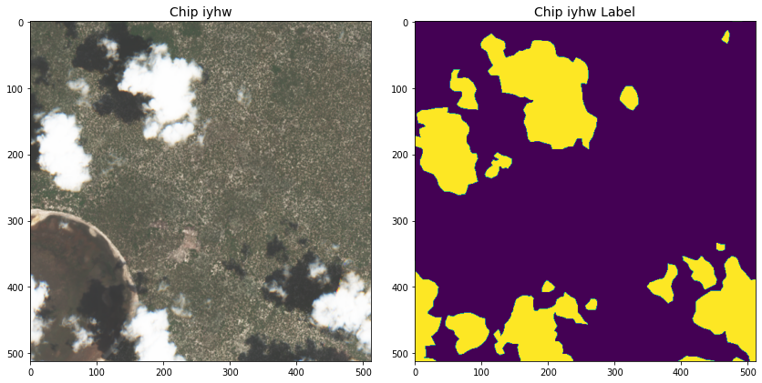
is cloud cover and purple is ground in this two-label setup.
DrivenData provided twelve thousand 512 x 512 GeoTIFF chips of training data, collected between 2018 and 2020, with four image bands per chip (see Table 1), metadata, and handcrafted labels. The labels were created by a 2021 Radiant Earth Foundation contest, and were later refined with expert annotators from TaQadam.
Provided Sentinel-2 Data Bands
| Band | Description | Center wavelength |
|---|---|---|
| B02 | Blue visible light | 497 nm |
| B03 | Green visible light | 560 nm |
| B04 | Red visible light | 665 nm |
| B08 | Near infrared light | 835 nm |
Despite these refinements, there appeared to be somewhere between five and ten percent of the chips with partially or fully incorrect labels, as figure 3 below illustrates.
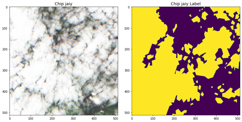
This sets the challenge for this competition. Train a model which is robust to incorrectly labeled data, but not too robust as to score poorly on the test set, which probably has a similar five to ten percent label error.
# Solution Summary
Code to reproduce this solution is available here.My solution was a customized version of XResNeXt50—the fastai version of ResNeXtSaining Xie, Ross Girshick, Piotr Dollar, Zhuowen Tu, and Kaiming He. 2017. Aggregated Residual Transformations for Deep Neural Networks. In Proceedings of the IEEE Conference on Computer Vision and Pattern Recognition (CVPR). with architectural improvements from the Bag of TricksTong He, Zhi Zhang, Hang Zhang, Zhongyue Zhang, Junyuan Xie, and Mu Li. 2019. Bag of Tricks for Image Classification with Convolutional Neural Networks. In 2019 IEEE/CVF Conference on Computer Vision and Pattern Recognition (CVPR), 558–567. DOI:10.1109/CVPR.2019.00065 paper—as the backbone for a customized DeepLabV3+Liang-Chieh Chen, Yukun Zhu, George Papandreou, Florian Schroff, and Hartwig Adam. 2018. Encoder-Decoder with Atrous Separable Convolution for Semantic Image Segmentation. In Computer Vision - ECCV 2018, 833–851. DOI:10.1007/978-3-030-01234-2_49 trained on five-fold split of the entire dataset.
# Model Specification
My customized XResNeXt50 architecture replaced all ReLU activation functions with with the MishDiganta Misra. 2019. Mish: A self regularized non-monotonic neural activation function. arXiv:1908.08681. activation function and the pooling layers with MaxBlurPoolRichard Zhang. 2019. Making Convolutional Networks Shift-Invariant Again. arXiv:1904.11486.. Instead of using a standard attention module, such as Squeeze and Excitation, I found the efficient combination of channel and spatial attention from Shuffle AttentionQing-Long Zhang and Yu-Bin Yang. 2021. SA-Net: Shuffle Attention for Deep Convolutional Neural Networks. arXiv:2102.00240. achieved better performance while only requiring a moderate increase of compute and memory during training.
DeepLabV3+ received fewer modifications. I replaced all the ReLU activation layers with Mish, but otherwise left the architecture at its defaults.
# Pretraining
Imagenet pretrained models work well as a base for transfer learning when the domain is similar to Imagenet. The further away from Imagenet the new domains get, the less practical use Imagenet weights have on downstream tasks. However, having a pretrained backbone is still useful for segmentation, especially with DeepLabV3+, its default settings have a lot of dropout.
Sentinel-2 imagery is a large enough domain shift from Imagenet that I personally observed little benefit of using an Imagenet pretrained model verses a model architecture I chose with my own pretrained weights.
After some experimentation, I pretrained the XSA-ResNeXt50 model to predict the ordinal classificationThe ordinal labels were generated on the fly from the transformed segmentation labels via a custom transform detailed below., zero through twenty, of cloud coverage on 256-pixel random crops from the 512 image chips using BCE loss.
The XSA-ResNeXt50 backbone was trained for 15 epochs at a learning rate of , on a batch size of 64, with a weight decay of , with the RangerLess Wright. 2019. New Deep Learning Optimizer, Ranger: Synergistic combination of RAdam LookAhead for the best of both. (August 2019). Retrieved from https://lessw.medium.com/new-deep-learning-optimizer-ranger-synergistic-combination-of-radam-lookahead-for-the-best-of-2dc83f79a48d optimizer, using cosine decay from fastai’s fit_flat_cos starting at seventy-five percent of total training steps.
In addition to random crops, I used a small amount random zoom, warp, 45 degrees of rotation, flipping, channel dropout, and random noise. I did not use any lighting or other color shifting augmentations, as I observed a significant decrease in model performance. Augmentation details can be seen in the DataBlock appendix.
I selected the best performing epoch via F1 Score, which was ~0.93 for all five folds, as the backbone weights for training DeepLabV3+.
# Training
After pretraining the custom XSA-ResNeXt50 backbone, I train the lightly modified DeepLabV3+ on the segmentation labels. To fit on the GeForce RTX 3090’s 24GB of RAM, I once again trained on 256 pixel random crops from the 512 pixel chips. I used a combination of label smoothing cross entropy loss and dice loss. Validation was conducted on 256-pixel four corner crops.
Similar to pretraining, the DeepLab model was trained for 80 epochs at a learning rate of , on a batch size of 64, with a weight decay of . Once again, I used Ranger as the optimizer with cosine decay starting at fifty percent of total training steps.
Likewise, in addition to random crops, final training used a small amount random zoom, warp, 45 degrees of rotation, flipping, channel dropout, and random noise. Augmentation details can be seen in the DataBlock appendix.
I selected the best performing epoch via Jaccard, which was between 0.894 and 0.905 across all five folds.
# Submitting Predictions
Predictions on the test set were largely unchanged. The one exception: predictions were generated on the whole 512-pixel chips rather than the 256-pixel four corner crops after I noticed a very slight increase in validation scores. This also removed some artifacts around the edges of the 256 crops when combining for the final 512 image.
This training and prediction procedure scored a Jaccard of 0.8712 on the hidden test set, a negligible shift from the results on the public test set, but a decline from the model’s validation five-fold Jaccard of 0.894 to 0.905. It is also behind the leader’s model score of 0.8974.
# Model Development Process
My solution was limited in part by compute availability. All my initial model development was done on Colab Pro and Kaggle Tesla P100 instances. These instances are slow. A training epoch on the full dataset, ~145 steps at a batch size of 64, took approximately 9 minutesWith validation each epoch took 9.75 to 10.5 minutes depending on instance variance.. Additionally, I needed to design my solution to fit on a P100’s 16GB of RAM.
I settled on the DeepLabV3+ model early on due to these limitations, as DeepLab is an architecture which combines accuracy and memory efficiency, due to the large amount of dropout in the default configuration.
My strategy was to create a subset of the training data to try out potential solutions on firstIf the task supports it, working on a subset is often a good idea as it allows for faster iteration with quick feedback., before scaling up to the entire dataset. Using this subset, I experimented with different model specifications, augmentations, weight decay, dropout, and optimizers, just to name a few.
A concrete example where this proved useful was pretraining. Initially, I iterated on a few different pretraining setups as a regression problem before switching to my solution’s ordinal classification procedure.
It was necessary to scale the best performing experiments up to the full dataset to validate their results. As expected, some hyperparameters which worked well on a subset did not scale to the full dataset.
The final five-fold model was trained on a rented 3090 from vast.ai at an out-of-pocket cost of approximately $12.
# Additional Experiments
After creating my top performing solution, I still had another two weeks until the competition finished. A short time thereafter I was able to acquire additional compute at a reasonable cost, so my ability to experiment increased.
However, my ability to submit solutions decreased at the same time. DrivenData did not have enough compute to process all the submissions at the end of the competition. The competition allowed for three submissions every twenty-four hours, but in the last two weeks DrivenData at its best only had enough compute to process one submission per contestant every eighteen hours.
This meant I had to be selective about which additional experiments highlighted below I scored on the test set.
# Fine Tuning at 512
The first additional experiment was an obvious one: fine tuning the 256-pixel crop model on the full size 512-pixel chips. However, all my experiments with fine tuning resulted in a degradation of performance on the validation set. I did not submit any of these models to be scored.
# Training on 384 Crops
I also trained on 384-pixel crops, with predictions on both 384 overlapping corners and full 512-pixel predictions. But my validation scores did not increase, so I decided not to submit any of these models.
# Training on 512
I submitted a model trained on the full 512-pixel chips. However, as this was a four-fold increase in computational cost, I could not train this model for as many epochs and it ended up scoring slightly lower on both the validation and test set. With hindsight, I suspect figuring out how to train this specification longer despite my compute limits was a better path to explore.
# Transformer Architecture
I also attempted to use alternative compute efficient segmentation architectures. I was interested in adding a transformer-based segmentation model and settled on SegFormerEnze Xie, Wenhai Wang, Zhiding Yu, Anima Anandkumar, Jose M. Alvarez, and Ping Luo. 2021. SegFormer: Simple and Efficient Design for Semantic Segmentation with Transformers. arXiv:2105.15203.. I followed the same strategy of pretraining the MiT backbone on ordinal classification and then training the full segmentation model on the cropped chips.
Unlike my DeepLab models, training SegFormer models resulted in very unstable validation. I am not sure if SegFormer is more sensitive to the label errors then my ResNet-DeepLab model, if I made an undetected error in my training recipesEven when following the SegFormer paper’s training procedure as closely as possible., or if there wasn’t enough data to train a transformer-based segmentation model.
Oddly enough, training the MiT backbone was easy and straight forward. It scored a similar F1-Score as my XSA-ResNet50.
# Pseudo Labeling
While training the above models, I also experimented with pseudo labeling the most incorrect labels. Inspired by Are we done with ImageNet?Lucas Beyer, Olivier J. Hénaff, Alexander Kolesnikov, Xiaohua Zhai, and Aäron van den Oord. 2020. Are we done with ImageNet? arXiv:2006.07159.—where Beyer et. al. removed the ten percent of the images with the highest loss and observed greater accuracy on the untouched validation set—I removed chips where the generated pseudo label appeared to be just as poor as the original.
This procedure required me to verify as best I could the new pseudo labels, and thus I limited it to the ~350 chips with the highest loss per fold. I kept the original label when it appeared accurate, generated a pseudo label if it looked accurate and the original label was inaccurate, and tossed the chip if neither the pseudo nor original label looked accurate. I repeated this procedure twice, using a model trained on the first round of pseudo labels to generate the second set.
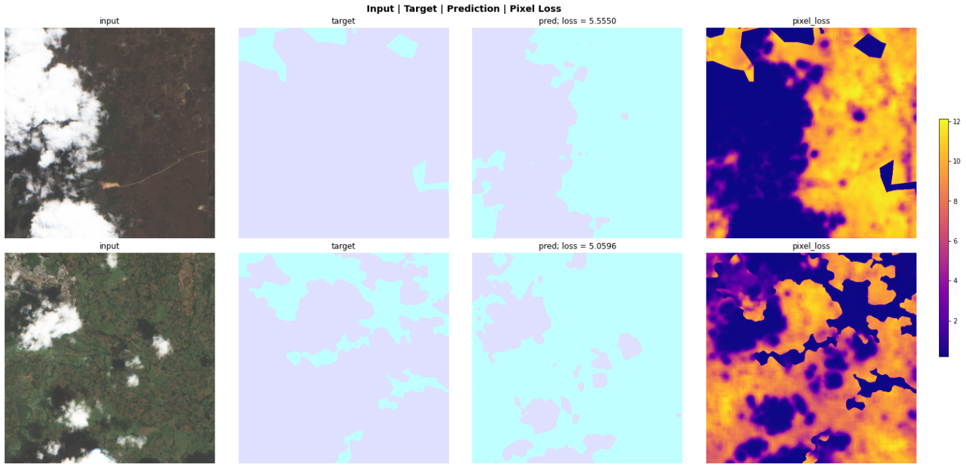
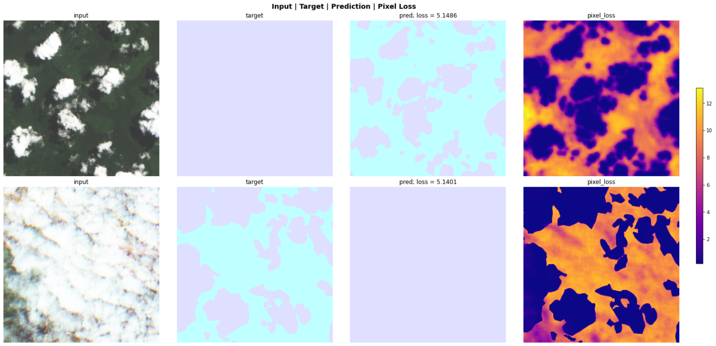
Figures 4 and 5 show a sample of four chips with labels which appear incorrect to my non-expert eye and a more accurate looking predicted pseudo labelPlots from an in-progress version of SegmentationInterpretation which will be added to the fastai dev build soon..
My intuition for this process was a model which is good at segmenting cloud cover is going to create “poor predictions” for the inaccurately labeled chips no matter what. But by fixing these labels, the model could learn a better representation and hopefully create better segmentation masks for the chips with accurate labels. Thus performing better overall against the test set.
Unfortunately, that is not what happened in practice.
These models had smoother training process, with less variation of validation loss and metrics. They scored better on the pseudo labels, with an average Jaccard of ~0.93 across all five folds while still scoring a similar Jaccard between 0.89-0.9 on the original labels.
However, when scored on the test set, the models trained on the pseudo labels performed significantly worse than those trained on the original labels.
# Conclusion
DrivenData has not released the test set yet, but with the benefit of hindsight, I expect one or two changes could have improved my solution relative to the leaderboard.
First, I think figuring out a method to train on the full chips for a longer amount of time could have resulted in a better performing solution. Second, I think my use of random crops probably hurt the solution’s attention to detail. I suspect a better crop selection strategyI have a few ideas, but will leave them for my next satellite imagery competition. would have improved the model’s performance.
# Appendix: Customizing fastai
This section assumes you have some familiarity with the internals of fastai including DataBlocks, Callbacks, transforms, and patching.Fastai doesn’t have native compatibility to open and process GeoTIFF filesAt least in the format used for this competition.. None of the existing DataBlocks will work. So, I needed to create a new DataLoader pipeline.
The fastai DataLoader pipeline for images can be broken down into six steps:
- Read an image into
PILImage(usually via a DataBlock) - Perform item transforms on
PILImage - Convert to
TensorImageviaToTensor - Batch all the
TensorImages - Convert to float via
IntToFloatTensor - Optionally, apply batch transforms to
TensorImage
For this project, I needed to create GeoTIFF compatible implementations for steps 1, 2, 3, and 5.
# New DataBlocks
The ImageBlock DataBlocks handles step 1 (read the image) and step 5 (convert from int to float).
First, I need to create a GeoTIFF compatible PILImage to handle step 1.
def _read_tif(fn):
    with rasterio.open(f'{fn}/B04.tif') as img:
        r_img = img.read(1).astype('float32')
    with rasterio.open(f'{fn}/B03.tif') as img:
        g_img = img.read(1).astype('float32')
    with rasterio.open(f'{fn}/B02.tif') as img:
        b_img = img.read(1).astype('float32')
    with rasterio.open(f'{fn}/B08.tif') as img:
        i_img = img.read(1).astype('float32')
    return np.stack([r_img, g_img, b_img, i_img], axis=0)

class TensorImageGeo(TensorImage):
    @classmethod
    def create_tif(cls, fn, **kwargs)->None:
        "Open an `Image` from path `fn`"
        return cls(torch.from_numpy(_read_tif(fn)))

    @classmethod
    def create_npy(cls, fn, **kwargs)->None:
        "Open an `Image` from path `fn`"
        return cls(torch.from_numpy(np.load(f'{fn}.npy')).float())
Unlike fastai’s PILImage, TensorImageGeo does not read into a pillow Image object. Rather it converts the read numpy array into a float32 PyTorch tensor.
This is for two reasons. First, pillow has known issues with processing and applying transforms to high-bit depth images and fastai’s item transforms use pillow as the backend. Second, PyTorch’s interpolateNeeded for item resizing in some specifications. doesn’t work on non-float data types.
Inheriting from TensorImage, means TensorImageGeo supports all of fastai’s data vis and plotting features. For brevity, I did not show the modifications required to plot TensorImageGeo via TensorImage.showThe competition GeoTIFF images are between 0-27600, instead of the expected 0-255 of 8bit RGB images., that code can be seen in the entire solution here.
With the new TensorImageGeo defined, I can now create a new DataBlock for it:
def GeoImageBlock(cls=TensorImageGeo, tif=True):
    if tif: return TransformBlock(type_tfms=cls.create_tif)
    else:   return TransformBlock(type_tfms=cls.create_npy)
I don’t include the IntToFloatTensor transform from step 5 as my TensorImageGeo is already a float tensor.
For reading the mask from GeoTIFF, I similarly create a TensorMaskGeo for my segmentation masks.
# Transforms
With the DataBlock defined, next I need to create transforms for steps 2, 3, & 6Step 5 is not needed as TensorImageGeo is already a float tensor..
Since TensorImageGeo inherits from TensorImage, all the existing batch image transforms will work out of the box with TensorImageGeo. The only thing I would need to do is implement batch image augmentation not covered by the base libraryI did create some custom image augmentations, but will not cover them here.. However, I do need a new transform for my pretraining labels. But first, setting up item augmentations.
# Patching Existing Augmentations
fastai has an extensive set of item augmentations which all use pillow as the backend. I previously created patches to extend these item transforms to support tensors as part of my fastxtend package. This covers step 2 (apply item transforms).
Since TensorImageGeo already is a Tensor, the ToTensor transform in step 3 is not needed. I created a patch for ToTensor so TensorImageGeo returns itself.
@ToTensor
def encodes(self, o:TensorImageGeo): return o
# New Transforms
Fastai automatically batches the Geo Images (step 4), the DataBlock handles step 5 (convert to float tensor) so the only thing that remains is custom batch transforms.
For pretraining, I wanted my labels to be the percent of cloud cover of random crops projected onto 20 ordinal classes. I also needed these labels to be accurate post affine transforms.
The easiest way to accomplish this is via a new batch transform: MaskToMultiClass.
class MaskToMultiClass(DisplayedTransform):
    order=100

    def encodes(self, x:(TensorMaskToClass, TensorCropMaskToClass)):
        s = x.shape
        x = x.sum(axis=(1,2)) / (s[1]*s[2])
        y = torch.zeros([x.shape[0], 20], dtype=x.dtype, device=x.device)
        for i in range(len(x)):
            z = torch.ones(int(20 * x[i]), dtype=x.dtype, device=x.device)
            z = F.pad(z, [0, 20-z.shape[0]])
            y[i] = z
        return TensorMultiCategory(y)

    def decodes(self, x:TensorMultiCategory):
        f = to_cpu if x.device.type=='cpu' else noop
        return f(x.sum(dim=1))
I will briefly explain MaskToMultiClass from top to bottom. MaskToMultiClass inherits from DisplayedTransform so it will always be appliedIn contrast, RandTransform is randomly applied at a probability of p.. The order=100 of MaskToMultiClass insures that it will run after all the affine transforms are applied to the segmentation mask. encodes uses fastcore’s type dispatch to only apply to TensorMaskToClass and TensorCropMaskToClass:
class TensorMaskToClass(TensorMaskGeo):
    pass
which are simple classes to ensure the transform is only applied to data I intended. For display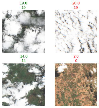
decodes used via show_results. Prediction on top, generated label on bottom. purposes, encodes returns a TensorMultiCategory to allow the new label to be plotted.
This occurs via the new decodes I added, which only applies to TensorMultiCategory via type dispatch and transforms the ordinal output to a readable number; and also required a patch to show to modify TensorMultiCategory to behave as fastai expected.
@patch
def show(self:TensorMultiCategory, ctx=None, **kwargs):
    "Show self"
    return show_title(str(self.item()), ctx=ctx, **merge({'label': 'text'}, kwargs))
For convenience, I created a GeoMultiClassBlock to automatically apply the MaskToMultiClass when pre-training my ordinal classifier. This implements step 6 (optional batch transforms) for the labels.
def GeoMultiClassBlock(cls=TensorMaskToClass, codes=None, tif=True):
    if tif: return TransformBlock(cls.create_tif, batch_tfms=MaskToMultiClass)
    else:   return TransformBlock(cls.create_npy, batch_tfms=MaskToMultiClass)
# Callbacks
When validating, my solution predicted four 256-pixel cropsAs I mentioned earlier, at test time I ended up predicting on the full 512-pixel image so this callback was unnecessary., but I wanted the loss and metrics calculated on the entire 512-pixel chip. The simplest way to accomplish this is via a Callback created to run after the predictions are generated, but before the validation loss is calculated.
CombineGeoCallback below combines the prediction crops into one prediction.
from torchvision.utils import make_grid

class CombineGeoCallback(Callback):
    run_train,order = False,MixedPrecision.order+1

    def after_pred(self):
        preds = []
        for i in range(0, find_bs(self.learn.pred), 4):
            preds.append(make_grid(self.learn.pred[i:i+4], nrow=2, padding=0))
        self.learn.pred = TensorImageGeo(torch.stack(preds, dim=0))
It’s set to only run on validation and after fastai’s MixedPrecision callbackMixedPrecision trains the model using PyTorch’s Automatic Mixed Precision.. In after_pred, it uses torchvision’s make_grid to combine every four predictions into one segmentation mask and assign them back to self.learn.pred. Then the loss and metrics can be calculated.
# Customizing fastai Conclusion
This has been a quick overview of how you can customize fastai when working on a new, unsupported problem. As you can see, fastai’s api is flexible enough that most tasks can be accomplished with a few new DataBlocks, Callbacks, transforms, and/or patches.
This competition required all these custom pieces, which is usually the exception to the rule. Most tasksOutside of NLP tasks. If you are working on NLP with fastai I recommend looking into blurr. will only require a subset of these customizations.
# Appendix: New & Improved Features
While working on this competition, I ran into some areas of fastai that I thought needed a bit of elbow grease. So I created new fastai functionality to address them.
Some features, such as a memory efficient Interpretation implementation have been accepted into fastai and should be part of the 2.5.4 release. While others such as the SegmentationInterpretation plot top losses used for Figures 4 and 5, are still in progress on my end at the time of writing. The most notable feature, the Metrics refactor to allow for tracking individual losses, currently exists as a draft PR.
Other new functionality, such as new augmentations, a more flexible version of XResNet, and the MultiLoss features will be added to my fastxtend package.
By the time you read this, all of these features might already have been added to either fastai or fastxtend.
# Appendix: DataBlocks
Pretraining DataBlock:
batch_tfms = aug_transforms(flip_vert=True, max_rotate=45,
                            max_zoom=1.2, max_warp=0.1, max_lighting=0,
                            xtra_tfms=[ChannelDrop(channels=4), RandomNoise()])

DataBlock(blocks=(GeoImageBlock(tif=False), GeoMultiClassBlock(tif=False)),
          get_x=[ColReader('chip_id')],
          get_y=[ColReader('chip_id')],
          splitter=ColSplitter('valid'),
          item_tfms=RandomCrop(256),
          batch_tfms=batch_tfms,
          n_inp=1)
Segmentation Training DataBlocks:
batch_tfms = aug_transforms(flip_vert=True, max_rotate=45,
                            max_zoom=1.2, max_warp=0.1, max_lighting=0,
                            xtra_tfms=[ChannelDrop(channels=4), RandomNoise()])

block = DataBlock(blocks=(GeoImageBlock(tif=False), GeoMaskBlock(tif=False)),
                  get_x=[ColReader('chip_id')],
                  get_y=[ColReader('chip_id')],
                  splitter=ColSplitter('valid'),
                  item_tfms=RandomCrop(256),
                  batch_tfms=batch_tfms,
                  n_inp=1)

vblock = DataBlock(blocks=(GeoImageCropBlock(tif=False), GeoMaskBlock(tif=False)),
                   get_x=[ColReader('chip_id')],
                   get_y=[ColReader('chip_id')],
                   splitter=ColSplitter('valid'),
                   batch_tfms=Normalize.from_stats(*cloudn_stats),
                   n_inp=1)

dls = block.dataloaders(df, bs=bs, num_workers=min(8, num_cpus()))
vdls = vblock.dataloaders(df, bs=bs//4, num_workers=min(8, num_cpus()))
dls.valid = vdls.valid